A word about unwanted variability

Experiments are influenced by various variables: the one we are interested in, and many others. Variability in the data can be related to differences in technical or biological variables, such as the instrument used, genetic background, age, gender, etc.  Therefore, batch effects are frequently observed in gene expression datasets.   They can affect genes independently of the variable of interest (independent of cancer or normal states, for example) or not (the expression of a given gene might be influenced by the age of the patient and by the cancer).

Overlooking batch effects may lead to faulty conclusions. Especially if an unaccounted variable (a technical variable for example) is correlated with the variable of interest.  For example, let’s say you want to study the effect of a treatment and you process all your control samples on the same day and all your treated samples a week later.  Ideally, no technical variation would be seen between the two dates.  But if something happened,  distinguishing the effect of the treatment from the effect of the technical variation (in this experimental setup) would be quite difficult.   Analyzing the data may lead to erroneous conclusion regarding the treatment effects.  You could think, for example, that the treatment induces stress-related pathways while this would be, in fact, related to a different handling of the cells on the two dates. Remember, correlation does not imply causality.

To avoid this situation, one needs to carefully plan and design its experiment to minimize possible sources of variation and to balance uncontrollable differences in order to avoid confounding variables. Do not hesitate to discuss this with a biostatistician or bioinformatician BEFOREHAND.

Surrogate variable analysis (SVA)

However, on a day to day basis, you still need to work with “noisy” data.  Among the existing methods for batch correction some assume that the batches are known, while others try to discover and control the unmodeled variability. The latter is exactly what the surrogate variable analysis intends to do. SVA tries to identify “unknown” variability, i.e. the variability that you are not aware of. This method aims at controlling this variability by building surrogate variables which can be used in subsequent analysis (in linear models, for example).

It was developed in 2007 by Leek et al to deal with batch effect in microarrays. The algorithm has evolved since the original publication (Leek et al. 2008, Leek et al, 2012) and several variations are available depending on the context of the required analysis (svaseq for count data, supervised sva, frozen sva). It is now widely used for batch correction and is available as a R Bioconductor package (sva), as well as in other packages such as limma.  Note that SVA might not be appropriate if the question of interest involves a number of heterogeneous subgroups.

While several implementations exist, the general framework is the same : 1) remove the signal attributed to the outcome of interest (remember, it wants to find unknown variability) and identify the subset of genes only affected by the unmodelled variability, 2) perform a decomposition of this reduced expression dataset to construct the surrogate variables, 3) use the surrogate variables in subsequent analysis as “known” variables.  To achieve that, it uses two cool methods : linear model and decomposition.  My goal here is not to explain in details how SVA works as much as introducing those two approaches.

Linear model and decomposition

Linear model

With linear models, the goal is to estimate the parameters of the equation.  The general equation of the models is

Y_i = β₀ + β₁x_i + e_i  

The coefficients β are estimated by minimizing the error between the points (Y_i) and the output of the equation for x_i. In the context of gene expression, we assume that the expression is composed of different signals : baseline expression, biological effect, known batch effect, unknown variability effect and error.

gene_expression = baseline + biological_effect + known_batch + unknown_batch + error

It is thus possible to estimate the contribution of each variable, for example the effect of the biological condition.  For practical exemples, have a look at the limma’s package user guide.

Singular value decomposition

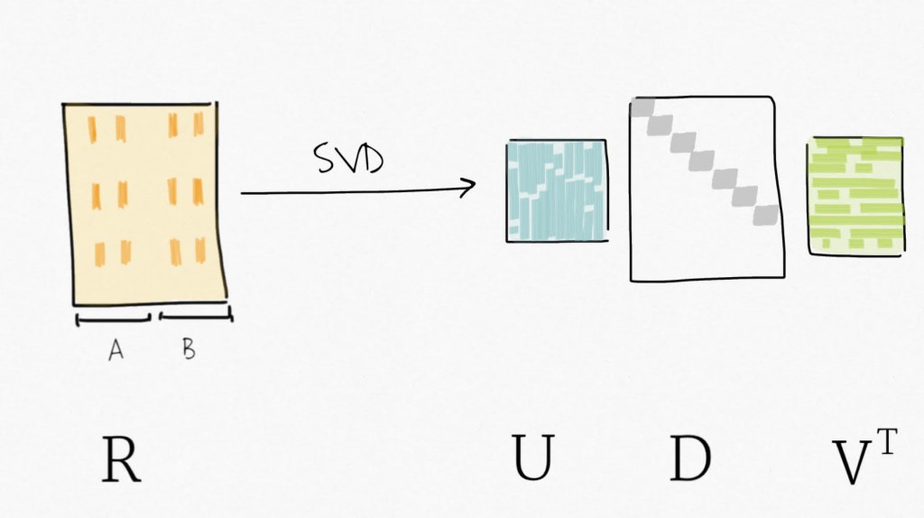
Singular value decomposition (SVD) can be seen as a dimensionality reduction technique.  SVD decomposes a matrix in three matrices : Y=UDV^⊤ . Precisely, for Y, a m x n matrix, SVD decomposes Y into U, an m x p orthogonal matrix  (left-singular vectors), V an p x p orthogonal matrix  (right-singular vectors, also sometimes referred to as eigengenes), and D a n x p diagonal matrix for p=min(m,n).  Simply put, SVD provides a way to compress the data in fewer variables sorted by decreasing variability (similar to what the Principal Component Analysis (PCA) does).

But “how is this related to SVA?” you might say…

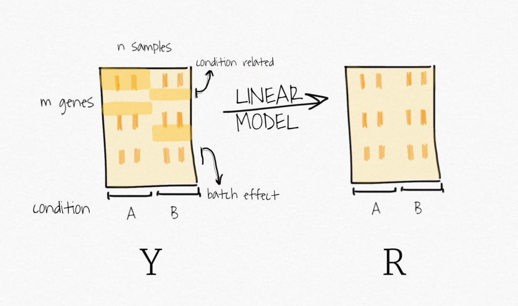
Well, to remove the signal attributed to the outcome of interest, SVA fits a linear model containing only the biological variable of interest.  It estimates the signal associated with this variable and then remove it from the data, to create a residual expression matrix.  Remember, the idea is to focus on unknown variability, it does not want to bias the following decomposition step toward the signal of this primary variable.

Then, applying SVD on the residual expression (no more signal attributed to the biological variable of interest) creates a set of variables ordered by decreasing variability.

The compressed variables allow the identification of subsets of genes only affected by these unmodelled variables.  These subsets are used to create reduced expression matrices.  Think of the subsets of genes as gene signatures in the residuals.

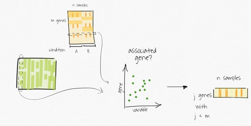
The decomposition of the reduced expression matrices provide the estimates for the surrogate variables which are used in subsequent analysis.

Other small notes here, the surrogate variables represent the collective unknown variability, they will not necessarily be associated with a specific variation source.  Also, the figures try to illustrate what I’m explaining in words.  They only serve the purpose of trying to make things clearer, they do not aim at being precise and accurate.  Have a look at the algorithms in the referenced papers for all the details.

Finally, I can not say if SVA is the best approach out there to correct batch effect.  But I hope you’ll have a broader understanding of batch correction in general with this small explanation of some key concepts.