Draw me a Circos

How pretty would that look in my article?
Very Pretty! As well as being informative!

You might want to use a Circos for your own personal analysis or as an article figure. In both cases, this kind of representation is useful when it comes to visualizing data in a more global or complete manner:  you can have multiple types of data ranging across various chromosomal sequences.

However, as wonderful and exciting the idea of having your own personal Circos might seem, for most of researchers, the path to get there is usually not hassle-free. For those whose best friend is not a computer, the concept of building your request (configuration files) and then feeding it to a console may seem abstract and, oh, so complicated.

Here are some tips, from my own usage of the software, that will hopefully make it easier for you to achieve the Circos of your dream.

Keep everything well organised and clear, and don’t be afraid of the <<include>> function.
Do not try to fit everything in one big configuration file! I have tried it and you will only get lost in all those lines (even if you are a top “commentator”). Instead, divide your files by blocks or parameters. For example, you could have a plots.conf file with everything relative to your 2D data tracks.

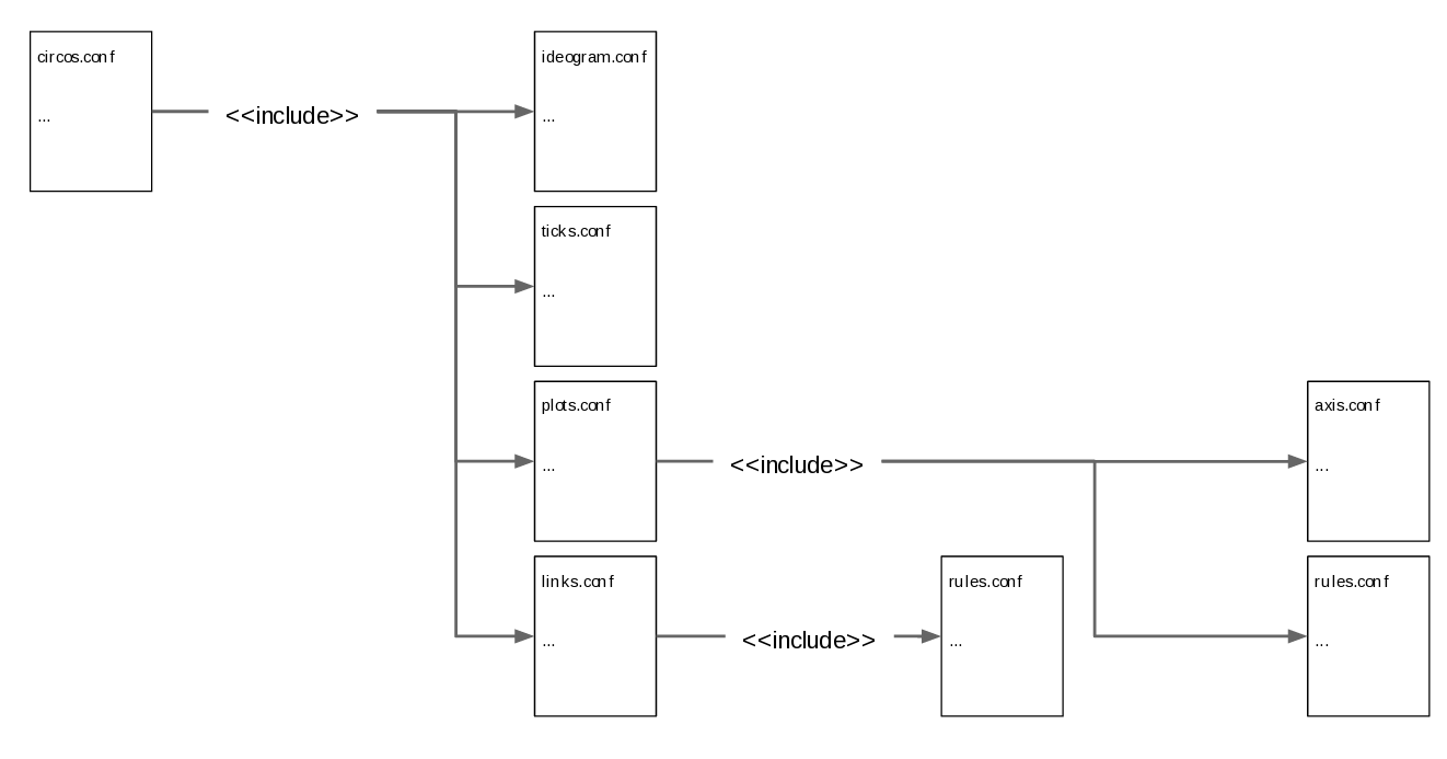
Make a “default” file (circos.conf), in which you declare the karyotype, chromosome(s) and file name(s), and include all the other files.
When it comes to rules, it is recommended to create a file only when there is recurrence. For example, if I am creating a rule specific to one plot, there is no need to create a file. However, if my rule applies to multiple plots, then I would create a rule.conf. Hence, instead of writing the entire block for every plot, I will just put “<< include rule.conf >>”.

Don’t try to get the perfect Circos on the first try.
Your first Circos should be a very simple one, to give you a big picture of all your data. Once you’ve got a good idea of what your results are telling you, you can personalize your image with colors, labels, emphasis on certain values, etc.

When doing your first analysis, use rules.
Rules block (<rules>) can be used in both plot and link blocks (<plot>, <link>). They are useful when you want to modify some data and/or values of your Circos without altering every links or the entire track. Let say that you are connecting regions containing similar sequences.  At first, it might not tell much, except that there are indeed similar sequences. The analysis could be deepened by, let’s say, only looking at sequences involving chromosome 1:

<links>
  <link>
    file = segdup.txt
    radius = 0.999r
    bezier_radius = 0.2r
    color = grey_a4
    thickness = 1.5
    <rules>
      <rule>
        condition = var(chr1) eq "chr1"  #link starts on chr1
        color = dred_a4
        thickness = 5
      </rule>
      <rule>
        condition = var(chr2) eq "chr1"  #link ends on chr1
        color = dred_a4
        thickness = 5
      </rule>
    </rules>
  </link>
</links>

 

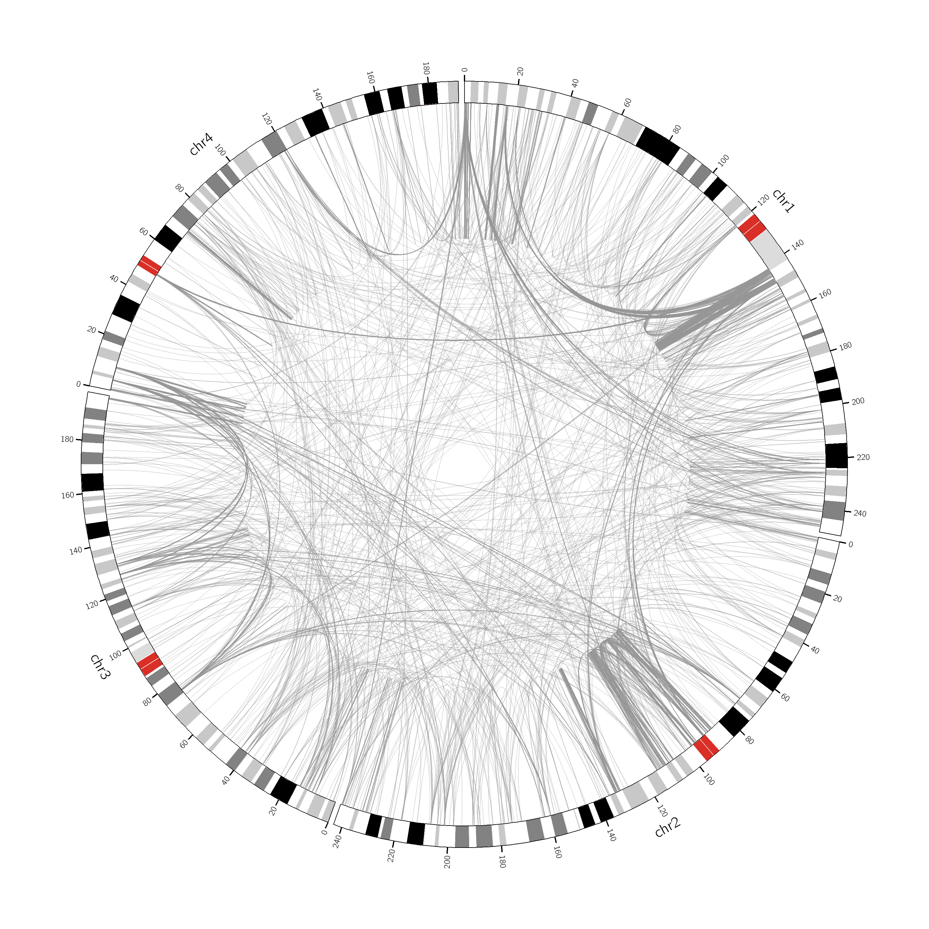
Sequence similarities between chromosomes 1, 2, 3 and 4

 

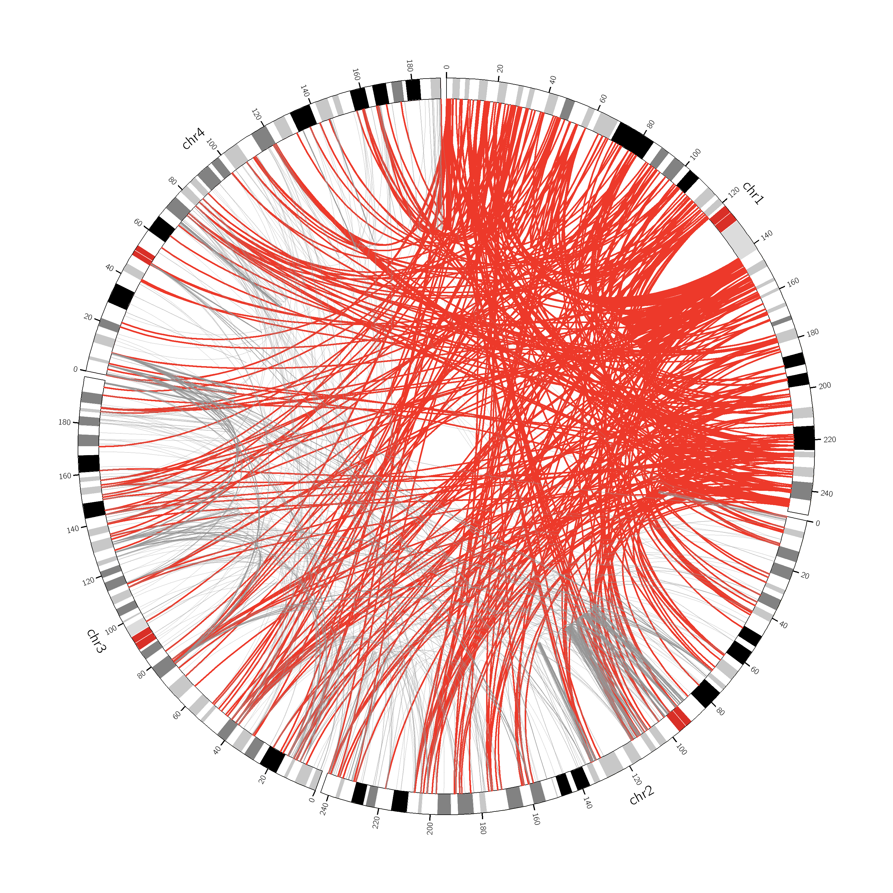
Sequence similarities between chromosomes 1 and 2, 3, and 4

Make good use of your space
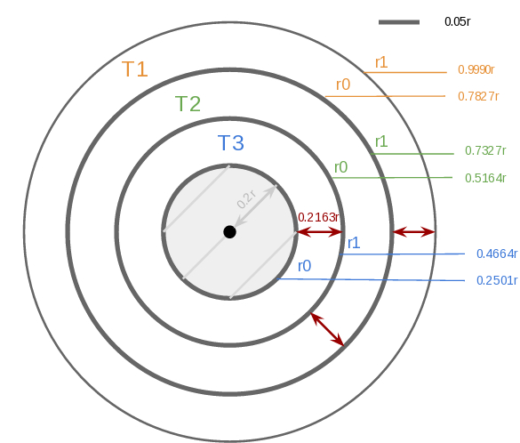
The hardest parameters to define are the track’s radius a.k.a r0 and r1. Keep in mind that you don’t have to get them perfectly on the first try. Therefore, I recommend you define a common width for all your tracks, with a very simple equation.

Where n is the number of track(s), p the desired padding between each track, s the innermost radius, e the outermost radius, and w the width.
Do not overcrowd your image with too many tracks and try to leave some space in the center since it gets harder to read and understand tracks near the center point. Let’s look at an example:

$n = 3$     $p = 0.05r$     $s = 0.2r$     $e = 0.999r$

$w = \dfrac{0.999r-0.2r-(3*0.05r)}{3} = \dfrac{0.649r}{3} = 0.2163r$

track 1:
r1 = 0.999r                                     

r0 = 0.7827r (0.999r – 0.2163r)

track 2:
r1 = 0.7327r (0.7827r – 0.05r)      

r0 = 0.5164r (0.7327r – 0.2163r)

track 3:  
r1 = 0.4664r (0.5164r – 0.05r)    

r0 = 0.2501r (0.4664r – 0.2163r)

Once you have your initial Circos, you can then tweak the radius values as you wish! For example, a tiles track does not need as much space as a histogram track.

 

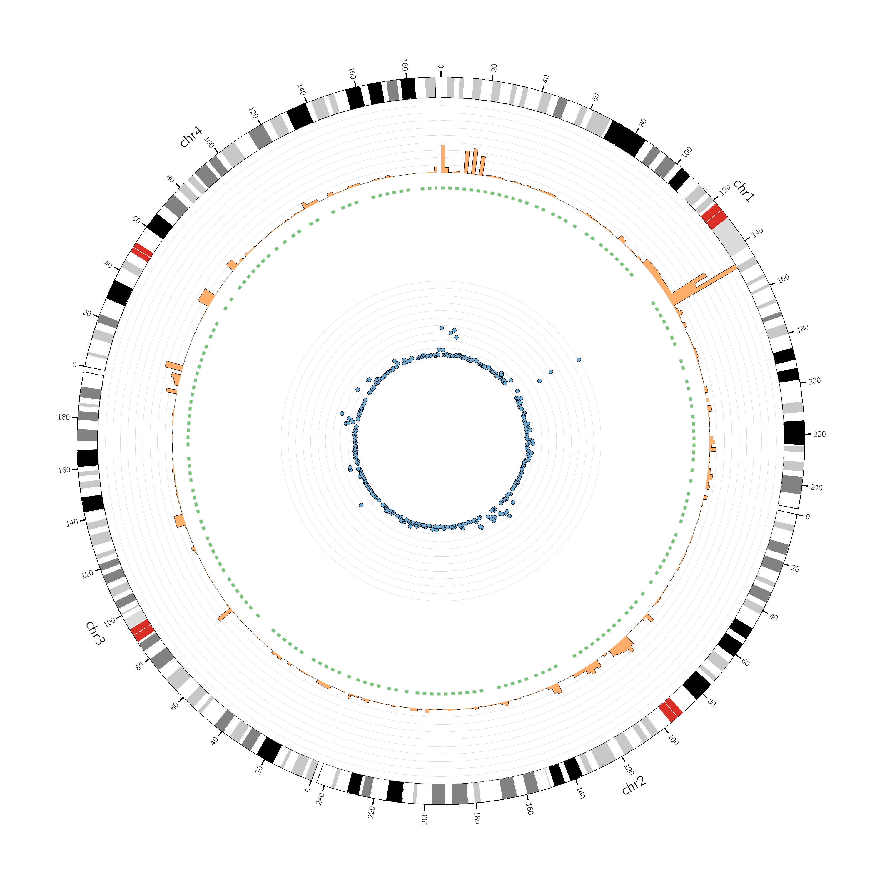
Circos with 3 tracks (histogram, tiles, scatter plot) of width w

 

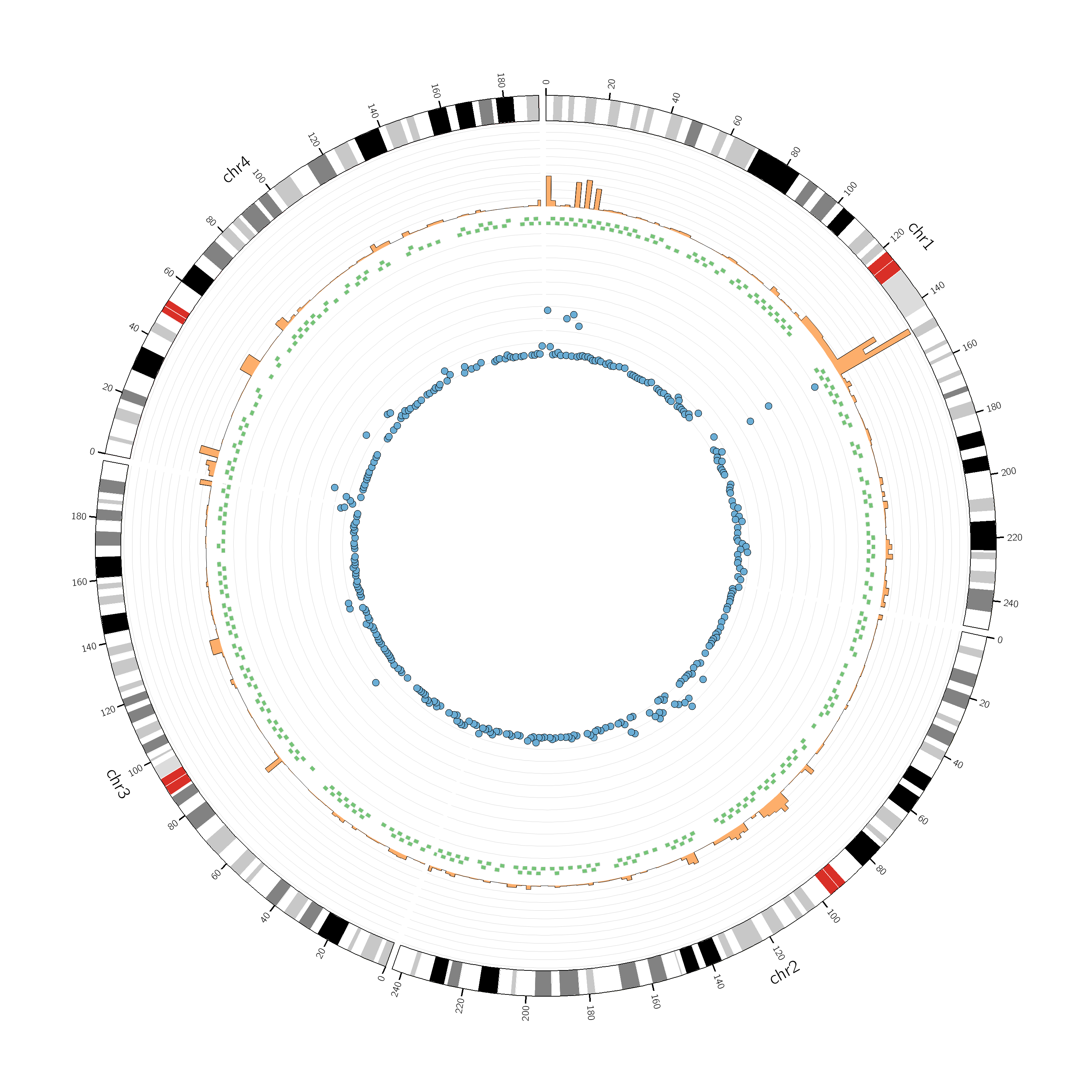
Circos with 3 tracks (histogram, tiles, scatter plot) of width w1, w2, w3

For more information you can refer to the Circos website and their tutorial tab.
You can also make use of our Circos user-friendly-interface!