Gradient descent is an iterative algorithm that aims to find values for the parameters of a function of interest which minimizes the output of a cost function with respect to a given dataset. Gradient descent is often used in machine learning to quickly find an approximative solution to complex, multi-variable problems.
In my last article, Introduction to Linear Regression, I mentioned gradient descent as a possible solution to simple linear regression. While there exists an optimal analytical solution to simple linear regression, the simplicity of this problem makes it an excellent candidate to demonstrate the inner workings of the gradient descent algorithm.
Cost function
Lets look back at the cost function outlined in Introduction to Linear Regression. This function represents the error observed while fitting our model onto the data. This is the error we would like to minimize. In this example, it corresponds to the mean of the vertical distance between our observations and the regression line squared (see Least Squares). In order to keep the size of the error manageable and to ensure that it won’t be affected by the size of our dataset, we divide by the number of observations (in essence calculating the mean of the errors).
$ Cost = \dfrac{\sum_{i=1}^n(y_i-(m x_i + b))^2}{N} $
Gradient
The gradient (the slope of our cost function at a given coordinate) represents the direction and the rate of change of our cost function. By following the negative gradient we are able to quickly minimize the cost function and arrive at a solution more rapidly. In order to obtain the gradient, our function must be differentiable with respect to the parameters we are trying to optimize. By taking the square of the distance we are guaranteed to have a positive output and a differentiable function.
The gradient is obtained by calculating the partial derivatives of our cost function with respect to the parameters $m$ and $b$ :
$ \dfrac{\delta}{\delta m} = \dfrac{2\sum_{i=1}^n-x_i(y_i-(m x_i + b))}{N} $
$ \dfrac{\delta}{\delta b} = \dfrac{2\sum_{i=1}^n-(y_i-(m x_i + b))}{N} $
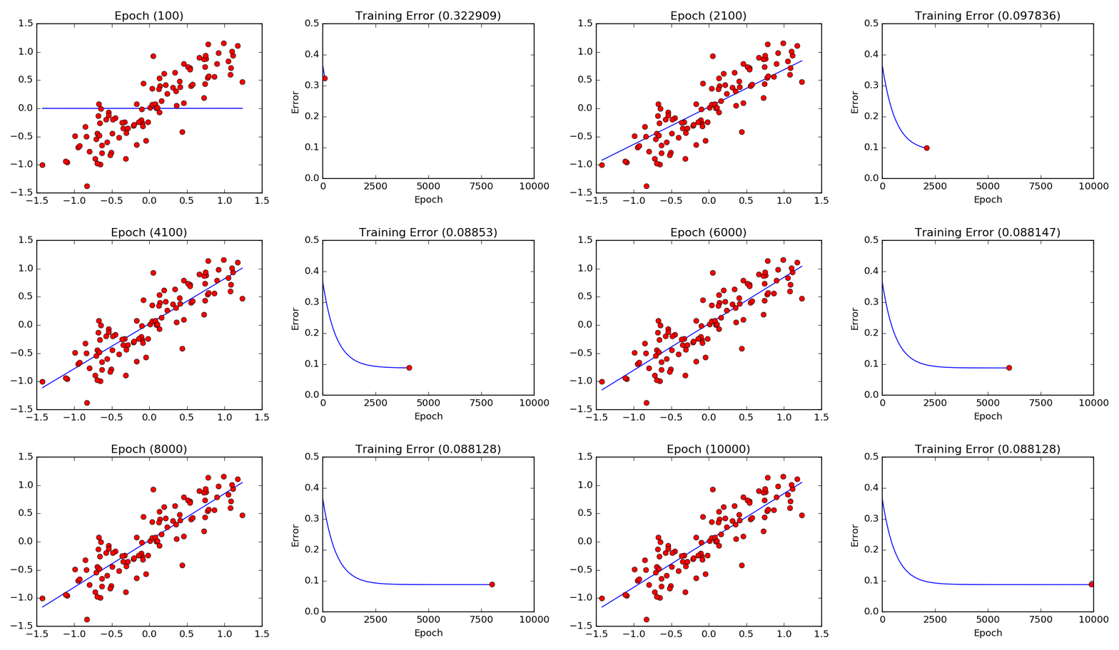
In gradient descent, two parameters must be fixed : the learning rate (the rate of change at each iteration) and the number of epochs (number of iterations/updates made during the gradient descent algorithm) during training. For this example, we will let gradient descent run during 10,000 iterations (epochs) with a learning rate (lr) of 0.001.
Code
import matplotlib.pyplot as plt
import numpy as np

# Cost Function
def error(m, b, X, Y):
    return sum(((m * x + b) - Y[idx])**2 for idx, x in enumerate(X)) / float(len(X))

# Gradient of Parameter m
def m_grad(m, b, X, Y):
    return sum(-2 * x * (Y[idx] - (m * x + b)) for idx, x in enumerate(X)) / float(len(X))

# Gradient of Parameter b
def b_grad(m, b, X, Y):
    return sum(-2 * (Y[idx] - (m * x + b)) for idx, x in enumerate(X)) / float(len(X))

def gradient_descent_LR(X, Y, epochs, lr):
    assert(len(X) == len(Y))
    m = 0
    b = 0
    for e in range(epochs):
        m = m - lr * m_grad(m, b, X, Y)
        b = b - lr * b_grad(m, b, X, Y)
    return m, b

if __name__ == '__main__':
    # Generate Noisy Dataset
    X = np.linspace(-1, 1, 100) + np.random.normal(0, 0.25, 100)
    Y = np.linspace(-1, 1, 100) + np.random.normal(0, 0.25, 100)

    # Run Gradient Descent
    m, b = gradient_descent_LR(X, Y, epochs=10000, lr=0.001)

    # Plot line using the values found by gradient descent for parameters m and b
    line_x = [min(X), max(X)]
    line_y = [(m * i) + b for i in line_x]
    plt.plot(line_x, line_y, 'b')
    plt.plot(X, Y, 'ro')
    plt.show()
Training Visualization

Gradient descent training visualization. Note that the parameters converge slower and slower as they approach their optimal values.
Another excellent article covering gradient descent in a bit more detail can be found at https://spin.atomicobject.com/2014/06/24/gradient-descent-linear-regression/.


Leave A Comment