

A data scientist’s first goal is to find underlying relations within the variables of a dataset. Several statistical and machine learning methods can be used to discover such relations. Once uncovered, this information can be applied to everyday problems. For example, in clinical medicine, a predictive model based on clinical data can help clinicians guide a patient’s treatment by offering insights that might not have otherwise been taken into account.
Simple linear regression
One of the most basic methods available to the data scientist is linear regression. The simplest case of linear regression is simple linear regression, linear regression with a single explanatory variable. Operating on a two dimensional set of observations (two continuous variables), simple linear regression attempts to fit, as best as possible, a line through the data points. Here, “as best as possible” means minimising the sum of squared errors, the distance between a point (an observation) and the regression line (see Least Squares). What purpose does this serve? The regression line (our model) becomes a tools that can help uncover underlying trends in our dataset. Furthermore, the regression line, when properly fitted, can serve as a predictive model for new events.
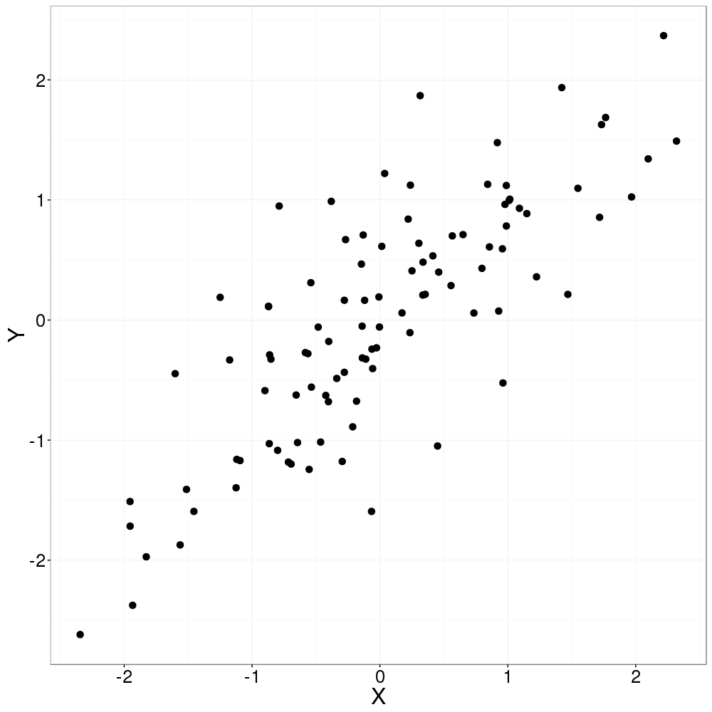 Scatterplot of our dataset. |
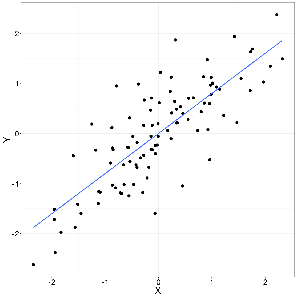 Fitting of the regression line (blue). |
While it may be tempting to use this line to predict events outside of the range of our observations (for example, events in the future based on historical trends), it is important to remember that this model can only reliably inform about the space from which it was built.
Task
A little more formally described, linear regression attempts to find the slope $m$ and intercept $b$ for a line which minimises the sum of errors (distances) squared between our observations and the line. Recall the general line equation :
$ y = m x + b$
It is worth noting that, while the perpendicular distance between a point and the line represents a more precise distance, it is the vertical distance which is used when calculating the error (or cost).
Naive Approach
Warning! This section and the code contained within is offered simply as a toy example. Proceed to the “Analytical approach” for a proper solution!
Knowing the line equation, could we not simply generate a large number of lines with different slopes and intercepts and hope to eventually find one that fits our dataset? Calculating the sum of squared distances would give us a metric for the fit of our line and the best one could simply be kept. Unfortunately this is a rather ambitious task. The search space is infinitely large! An infinity of lines must be generated in order to find an optimal solution. Even if we content ourselves with a non optimal solution, this technique would realistically only work if we drastically restrict the search space.
Who said we needed a logical reason to code something anyway? Here is an implementation of this silly approach in Python :
import random

def error(m, b, X, Y):
 assert(len(X) == len(Y))
 return sum(((m*x+b) - Y[idx])**2 for idx, x in enumerate(X))

def naive_LR(X, Y, n):
    assert(len(X) == len(Y))
    best_error = None
    best_m = None
    best_b = None
    for i in range(0,n):
        # Warning! the ranges for m and b must be selected
        # carefully based on the values contained in the dataset.
        m = random.uniform(-100, 100)
        b = random.uniform(-100, 100)
        error = error(m, b, X, Y)
        if error < best_error:
            best_error = error
            best_m = m
            best_b = b
        return best_error, best_m, b
Surprisingly enough, this code arrives to a rather well fitted line during some tests. It is clear however, that the success of this code depends heavily on the search space ranges given for $m$ and $b$. Here, the ranges were chosen more or less arbitrarily, making sure to select values well outside the maximum ranges of our dataset. Of course, far better heuristics can be elaborated to select more appropriate ranges based on a given dataset (with the unfortunate side effect of rendering this solution much less naive). Finally, the number of lines to be generated, $n$, must also be fixed. The number of lines generated raises the chance of finding a well fitted line, as well as the computing time.
Analytical Approach
Luckily, this type of problem is simple enough to warrant a purely analytical solution. As described earlier, it is the sum of the vertical distances squared that we are using as cost function and which we are hoping to minimise. This cost function is defined as such :
$ cost = \sum_{i=1}^n(y_i-\hat{y_i})^2 $
Inserting the line equation for the y value on the regression line we get :
$ cost = \sum_{i=1}^n(y_i-(m x_i + b))^2 $
A bit of manipulation allows us to separate out the slope. Note that a bar placed on top of a variable (e.g. $\bar{x}$) represents the average in our observations for that variable.
$ \hat{m} = \frac{ \sum_{i=1}^n (x_i – \bar{x})(y_i – \bar{y}) }{ \sum_{i=1}^n (x_i – \bar{x})^2 } $
Once we solve for the slope, we can throw it to the line equation to retrieve the intercept $b$.
$ \hat{b} = \bar{y}-\hat{m}\,\bar{x} $
(A more verbose mathematical reasoning can be found in the wikipedia article for simple linear regression, as well as the notes for a statistics class from the university of florida.)
The code :
def mean(l):
    return float(sum(l)) / len(l)

def analytical_LR(X, Y):
    assert(len(X) == len(Y))
    mean_x = mean(X)
    mean_y = mean(Y)

    num = sum((X[idx] - mean_x)*(Y[idx] - mean_y) for idx in range(len(X)))
    denum = sum((X[idx] - mean_x)**2 for idx in range(len(X)))
    m = num / float(denum)
    b = mean_y - m*mean_x
    error = error(m, b, X, Y)

    return error, m, b
Iterative Approach – Gradient Descent
A solution can also be found by gradient descent. This method attempt to approach an optimal solution by adjusting, little by little, the parameters of the function to optimise. While it is possible to apply this method to simple linear regression, it is generally used for non linear regressions where an analytical solution would be computationally prohibitive or simply not available. Gradient descent is a method often used in machine learning when training neural networks. This method can rapidly obtain an approximate solution to complex problems.
This approach will be covered in a future blog post. Stay tuned!
Leave A Comment