

This series of articles on machine learning wouldn’t be complete without dipping our toes in overfitting and regularization.
Overfitting
The Achille’s heel of machine learning is overfitting. As machine learning techniques get more and more powerful (large number of parameters), exposure to overfitting increases.
In the context of an overfit, the model violates Occam’s razor’s principle by generating a model so complex that it begins to memorise small, unimportant details (with no true link to our target) of the training set. Such a model becomes so fine tuned to its training set that it cannot generalize to new samples. Luckily, overfitting can be mitigated through regularization techniques, allowing the generation of a more parsimonious model.
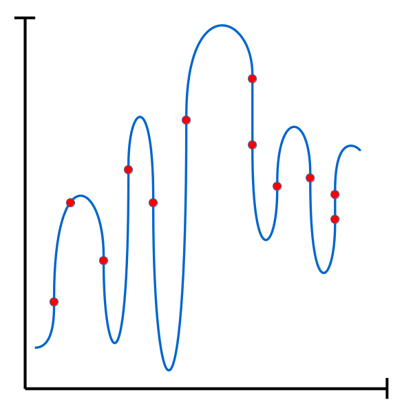 Typical case of overfitting. While the final function covers all the training set’s data points, it is likely that it would score poorly on new data as it fails to capture the underlying trend in the data. |
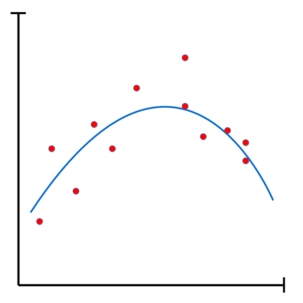 While this function has a higher overall error than the previous one, it offers a simpler and more general solution. This function is likely to perform better on new data. |
Regularization
Regularization aims to limit overfitting. While some regularization methods can be quite complex, some are strikingly simple. For example, a model can be forced to better generalize by simply limiting its capacity (number of parameters).
Early stopping
Mostly used in the context of gradient descent, early stopping attempts to pinpoint the precise moment when the model begins to overfit and halt training. To do this, a part of the training set is set aside as a validation set. This validation set, hidden from the model during training, is used to offer a more objective performance metric. Once the error on the validation set begins to raise, it can be said that the model has begun overfitting the training data.
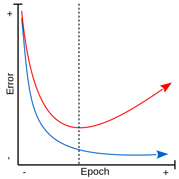 Learning (training) curves for training set (blue) and validation set (red). The dotted line marks the beginning of the overfit (inflexion point for the validation error) and the time at which training should be halted. |
L1 / L2
Regularization can also be applied directly to the cost function, as is the case with the L1 and L2 norms. Manipulating the error function in order to control overfitting is another popular method in machine learning.
Regularization by L1 norm (Lasso) attempts to minimise the sum of the absolute differences between real and predicted values ($\theta_i$). Linear, it offers the model the possibility to easily set weights to 0 and can therefore also be useful for feature selection by forcing a sparse representation.
$ L1 :\lambda\sum_{i=1}^n |\theta_i| $
Regularization by L2 norm (Ridge / Tikhonov) attempts to minimise the sum of the squares of the differences between real and predicted values ($\theta_i$). This term is slightly faster to compute than its cousin, L1. Exponential, it promotes a diffuse representation which tends to perform better than regularization by L1.
$ L2 : \lambda\sum_{i=1}^n \theta_i^2 $
Finally, the effect of the regularization is controlled by a weight variable ($\lambda$) placed in front of the term.
There you have it! I hope you were inspired by this little detour on the issue of overfitting and by some of the solutions offered by regularization. As always, stay tuned for updates in this series on machine learning!
Leave A Comment