Say we have the two following groups :
g1 <- c(55, 65, 58)
g2 <- c(12, 18, 32)
We want to see if the two groups belong to the same distribution or can be considered as different groups. We might be tempted to try a Student’s t-test.
t.test(g1, g2)## Welch Two Sample t-test
##
## data: g1 and g2
## t = 5.8366, df = 2.9412, p-value = 0.01059
## alternative hypothesis: true difference in means is not equal to 0
## 95 percent confidence interval:
## 17.34281 59.99052
## sample estimates:
## mean of x mean of y
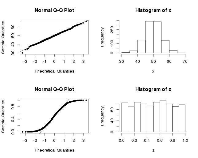
## 59.33333 20.66667The t-test gives a low p-value which indicates that there is a significant difference in means. But wait, are we allowed to use this statistical test? One of the assumption underlying the t-test is that your data has to follow a normal distribution. With three samples in each group, it’s hard to decide, based on the observations alone, if the distribution is normal. One standard visual way to assess if a dataset has a normal distribution is to do a Q-Q plot. It compares the data to the theoretical quantiles of the normal distribution. When the points are linear, it suggests that the data is normally distributed. Here are the Q-Q plots for x, which is normally distributed since it was built with the function rnorm, and for z which is uniformly distributed.
x <- rnorm(1000, mean=50, sd=5) # normal distribution
z <- runif(1000) # uniform distribution
par(mfrow=c(2,2))
qqnorm(x, pch=20)
qqline(x)
hist(x)
qqnorm(z, pch=20)
qqline(z)
hist(z)
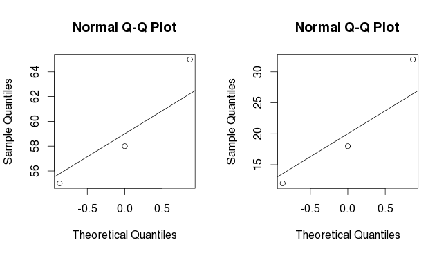
If we try to do the same with g1 and g2, we do not get much insight into the distribution of our data. We have too few points.
par (mfrow=c(2,2))
qqnorm(g1)
qqline(g1)
qqnorm(g2)
qqline(g2)
Without knowing the distribution, we might want to switch from a parametric statistic test to a non-parametric statistic test. The U-Mann-Withney-Wilcoxon test is a widely used non-parametric test. It compares the ranking of the values not the actual values themselves. I’ve explained the first steps of the test in a (previous post).
wilcox.test(g1, g2)## Wilcoxon rank sum test
##
## data: g1 and g2
## W = 9, p-value = 0.1
## alternative hypothesis: true location shift is not equal to 0The p-value obtained with the wilcox.test is higher than the p-value we had obtained before.
Here, you should be aware that the t-test and the u-test do not have the same null and alternative hypothesis. You’re not testing exactly the same thing. The t-test checks whether the true mean difference between the two groups is different from zero while the u-test tests whether a particular population tends to have larger values than the other, i.e. if the medians are equal. In the end, both tests are used to confirm whether two groups come from the same population but it’s good to know what hypothesis are actually tested. In the case of g1 and g2, we clearly see that the sample medians are not equal. The data supports a difference of medians. So, why is the u-test giving us an insignificant p-value of 0.1? Because we have too few samples!! The significance (in the critical values table of the Mann-Withney U) is not even defined for 3 versus 3 samples comparison. It’s surprising that we get a p-value at all in R.
Now what? What can we do? The first thing I would answer is: get more data!!! But if it’s impossible, we can try to use a permutation test. With small dataset, a complete permutation can be used to obtain the complete permutation distribution. For larger datasets (where enumeration of all permutations is not desirable), a sampled permutation test can be used. In this case, it’s important to pick combinations randomly and with an equal probability.
How does it work? First, we need to compute a statistic for our two groups: difference of medians, of means, of sums. This is your observed value, T(obs).
Then, we pool all the data and shuffle the associated labels (group1/group2). We compute the statistic for all permutations (or a number of n repetitions). When we are finished, we count the number of times the random statistic was better than our observed statistic. By definition, a p-value represents the probability that a test gives a result at least as extreme as observed under the null hypothesis (could be simply put as the probability that what you observed is observed by chance). Here, the null hypothesis becomes that the group labels are randomly assigned. So we have the probability of observing our statistic under the hypothesis that the labels had no importance.
Tobs <- sum(g1)-sum(g2)
data <- c(g1, g2)
combinations <- t(combn(data, 3, simplify=T))

diff <- function(data, combination_i=0, all_combinations=NULL) {
  # if we do not list all possible combinations, we pick random combination
  if (combination_i==0) {
    x1 <- sample(data, 3, replace=F)
  }
  # if we are listing all combinations
  else {
    x1 <- combinations[combination_i,]
  }
  # The random combination is assigned to group1; we assign the remaining values to group2
  x2 <- data[!data%in%x1]
  # We return the statistic
  return (sum(x1)-sum(x2))
}

Trand <- c()
# We list all combinations found using combn()
for (i in 1:nrow(combinations)) {
  Trand <- c(Trand, diff(data, combination_i=i, combinations=combinations))
}
sum(Trand>=Tobs)/nrow(combinations)
## [1] 0.05For sampled permutation test, replicate function is really useful to repeat an expression/function a number of times. Here, we chose randomly 3 values for the first group and put the remaining 3 in the second group. We repeated this 1000 times.
Since there is 20 combinations for group 1, (choosing 3 among 6=20; n!/k!(n-k)! where n is the total of choices and k the number you want to choose), we certainly chose the same combinations more than once in our 1000 repeats. We actually chose each combination 50 times on average.
# We do not list all the combinations, but we pick a random combination n number of times
# We can use the same function as before
n <- 1000
Trand <- replicate(n, diff(data=data))
sum(Trand>=Tobs)/n
## [1] 0.065The complete permutation test is probably the better choice in this case.
Permutations tests (and bootstrapping methods) are useful in many situations. The example I have showed here highlighted the problem of small datasets, but really the usage of permutations tests is not limited to this situation.
And lastly, remember that 3 samples is not a friendly number to do statistic tests ! Plan your work in consequence because you know what they say: better safe than sorry.


Leave A Comment