

GEO offers an extremely rich source of transcriptional profile data, but downloading and preparing a dataset is often an obstacle to aspiring bioinformaticians. I’ll walk you through one way to do it using the Leucegene dataset as an example. Once this data is loaded and ready to use in R, I’ll then present a very simplified and practical perspective on the use of PCA for exploratory analysis.
Loading data
A dataset of 285 transcriptional profiles of acute myeloid leukemia (AML) can be downloaded from GEO at this link (Accession: GSE67040). This cohort was sequenced (RNA-Seq) in the context of the Leucegene project (web site) and represents 285 patients. Once downloaded from GEO, the “GSE67040_RAW.tar” file can be expanded on a mac by double-clicking on it (on linux, you can use “tar xvf GSE67040_RAW.tar” to expand it). This results in 285 text files, each containing the expression of 24,553 genes. The files will look like this:
chr1 11874 14361 DDX11L1 0.04970 1400
chr1 14410 29370 WASH7P 1.95957 59227
chr1 69091 70008 OR4F5 0.00620 100
chr1 134773 140566 LOC729737 2.24401 215729
chr1 567705 567793 MIR6723 0.00000 0
To load a single file in R, we could use:
data <- read.delim ("GSM1636929_14H038_RPKM.txt", header=F, col.names=c("chr", "start", "end", "sym", "rpkm", "count"))
head (data)
chr start end sym rpkm count
1 chr1 11874 14361 DDX11L1 0.04970 1400
2 chr1 14410 29370 WASH7P 1.95957 59227
3 chr1 69091 70008 OR4F5 0.00620 100
4 chr1 134773 140566 LOC729737 2.24401 215729
To load all samples, we would loop over all file names fitting the given pattern and concatenate the resulting data frame, taking care to add a column identifying the samples from which the expression values are measured. The following few lines of code will run for 5-10 minutes (with the “rbind” being the culprit for this unjustifiable slowness, I’ll leave optimization up to the curious reader!):
all.fn <- list.files (pattern="GSM.*_RPKM.txt")
all.data <- data.frame()
data.len <- sapply (all.fn, function (fn) {
    pat <- unlist (strsplit (fn, "_"))[2] ## Extract the patient id
    data <- read.delim (fn, header=F, col.names=c("chr", "start", "end", "sym", "rpkm", "count"))
    data$pat <- pat                       ## Add a column identifying the patient
    all.data <<- rbind (all.data, data)   ## Accumulate the profiles in all.data
    nrow (data)                           ## I used this to verify that all profiles contained the same number of genes, see data.len
}
This data is presented in what is often called a long format: each row represent a single expression value and the first few columns identify the gene. Here, we will combine columns #1-4 to act as the gene name and keep column #5 as the expression value (measured in RPKM). To those familiar with ggplot2, you will recognize that this long format is the preferred one of this great graphing package. As an aside, it is also extremely convenient when working with “lm” and “glm”! But here, I will convert this format into a more traditional matrix format where rows represent genes and columns represent patients. This is sometimes referred to as a wide format and is easily performed using “acast” from the “reshape2” package (the reshape package provides functions to convert to and from long and wide formats). Finally, I’ll transform the RPKM values using the started-log transform.
library (reshape2)
z <- acast (all.data, chr + start + sym ~ pat, value.var="rpkm")
zl <- log10 (z + 0.001)
Principal component analysis (PCA)
Data is loaded and ready to be analyzed… but where to start? It is a good idea to spend some time exploring a new dataset in an undirected fashion. A great tool to apply for this purpose is the PCA. Although you’ll find numerous texts detailing the precise mathematical underpinnings of the PCA (I’ll refer the curious readers to the exhaustive presentation of Jolliffe 1986 (link)), I like to think of PCA as defining a series of gene signatures in which every gene has a specific weight. The first signature (called the first component in PCA jargon or PC1 in R) identifies the genes that can best differentiate samples of the dataset. If you would take each transcriptional profile and multiply gene expressions by the weights given by this first component and sum this into a unique score, this score would capture as much variance from the dataset as is possible using a single value. The second component (or signature) will be orthogonal to the first, meaning that it will capture variance that is independent from that captured with the first component. And so on with following components.
Using the PCA, we thus replace each transcriptional profile (24,553 gene expressions per sample) by a set of values (the scores describe above) in such a way that this transformation preserves the variations observed in the complete dataset.
pr <- prcomp (t (zl), center=T)
x <- predict (pr)
The “rotation” variable contains the signatures (components) as columns, and “predict” is used to compute the “scores” of those signatures for each of our samples.
plot (x[,c(1,2)], pch=20)
text (x[,c(1,2)], rownames (x))
With this type of representation, it is very easy to identify outliers. If samples fall into easily distinguishable classes, this would also show. To further show the usefulness of PCA as first exploratory step, the following piece of code will identify the samples corresponding to leukemias belonging to FAB classes M0-1 (M0 and M1 combined), M5 and M6. These types of leukemias are known to have somewhat characteristic expression profiles. The output of the PCA clearly shows that PC1 (the main PCA “signature”) defines characteristics of the M0-1 and PC2 allows to distinguish between M5 and M6.
p.M6 <- scan (what=character())
>>04H017 04H039 05H097 07H024 10H066 11H183 07H034 03H028 12H067 12H117
p.M5 <- scan (what=character ())
>>03H041 07H089 07H134 08H089 10H026 12H096 14H031 01H001 02H026 02H032 02H033 03H016 03H067 04H080 04H111 04H115 04H118 04H121 05H025 05H065 05H128 05H143 06H010 06H016 06H073 06H074 07H041 07H045 07H063 08H011 08H021 08H063 08H108 08H139 09H008 09H010 09H024 09H032 09H098 09H102 10H022 10H055 10H058 10H127 11H006 11H083 11H095 11H192 13H019 13H141 13H185 03H052 04H041 05H013 05H094 05H181 07H055 07H155 08H004 08H049 08H104 09H042 09H106 09H111 10H029 10H031 10H072 10H161 11H126
p.M01 <- scan (what=character ())
>>02H003 02H017 03H030 04H096 05H179 06H133 06H135 07H038 08H118 09H018 09H079 10H014 10H038 11H002 11H014 11H046 11H138 11H170 12H030 12H149 13H039 13H048 13H056 13H083 14H012 14H019 14H027 02H009 02H025 02H043 02H053 02H060 02H066 03H024 03H033 03H036 03H081 03H090 03H094 03H116 03H119 04H001 04H006 04H024 04H025 04H048 04H055 04H103 04H108 04H112 04H117 04H120 04H127 04H133 04H135 04H138 05H008 05H022 05H030 05H034 05H078 05H111 05H163 05H184 05H195 06H028 06H029 06H088 06H089 06H103 06H144 06H151 07H060 07H062 07H107 07H112 07H125 07H133 07H135 07H137 07H151 07H152 07H158 07H160 08H012 08H034 08H048 08H053 08H056 08H065 08H082 08H085 08H113 08H129 09H002 09H022 09H026 09H031 09H040 09H043 09H045 09H048 09H070 09H078 09H083 09H088 09H090 09H113 09H115 10H040 10H048 10H056 10H068 10H070 10H092 10H095 10H107 10H109 10H113 10H115 11H010 11H019 11H035 11H058 11H097 11H103 11H107 11H129 11H135 11H142 11H151 11H186 11H232 11H240 12H010 12H021 12H039 12H056 12H079 12H091 12H116 12H171 12H172 12H173 12H175 12H176 13H073 13H080 13H139 13H150 13H158 13H169 14H001 14H017 14H020
plot (x[,c(1,2)], pch=20)
points (x[(rownames (x) %in% p.M6), c(1,2)], pch=20, col="yellow")
points (x[(rownames (x) %in% p.M5), c(1,2)], pch=20, col="orange")
points (x[(rownames (x) %in% p.M01), c(1,2)], pch=20, col="blue")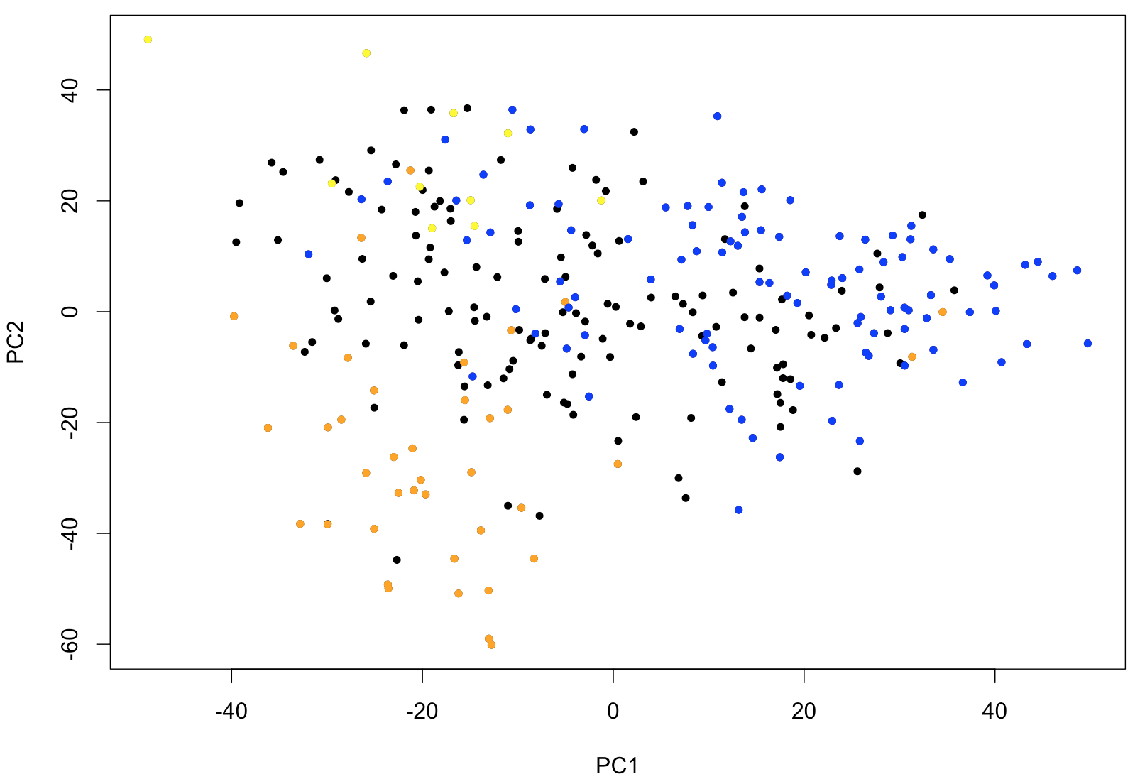
Figure 1: PCA of 285 patient samples from Leucegene shown using the first two principal components. Colors corresponds to FAB classification with M0 and M1 shown in blue, M5 in orange and M6 in yellow.
Leave A Comment