

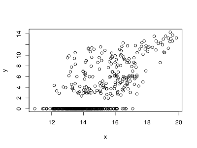
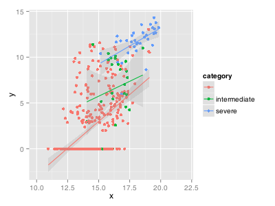
So you have spent much time converting your simple R plot to a full-fledged ggplot2 graph with all its bells and whistles just to find that you are unable to identify a point on this graph to further investigate it. Indeed, the typical identify method is not applicable to ggplot2 graphs.
Fortunately, there is a solution, which involves performing all the work yourself by going under the hood of ggplot2 to access the low-level graphics system on which it is built, namely grid. The grid package provides methods to divide a window into multiple graphics regions, each with its own viewport. We will then use these methods to access the plot viewport and perform the conversion between screen coordinates and data coordinates to identify the closest point.
There is in fact a hierarchy of viewports and after having created our plot, we need to find the appropriate one somewhere among all the others that represent the background, title, axis, legend, etc. In the simplest case, this viewport is fortunately typically named panel.3-4-3-4 and we move our reference coordinate system to this viewport like such:
qplot(x, y) + xlim(c(0,10)) + xlim(c(0.1,0.5))
downViewport('panel.3-4-3-4')
pushViewport(dataViewport(x, y, c(0,10), c(0.1, 0.5)))
We can then grab the screen coordinates (in inch, no less!) relative to the lower left corner of the plot using the grid.locator and then find the point from our data which is closest to these coordinates. To do so, we use the convertUnit methods to transform our data from their native values to inches.
pick.n <- as.numeric(pick)
view.x <- as.numeric(convertX( unit(x,'native'), 'in' ))
view.y <- as.numeric(convertY( unit(y,'native'), 'in' ))
w <- which.min((view.x-pick.n[1])^2 + (view.y-pick.n[2])^2)
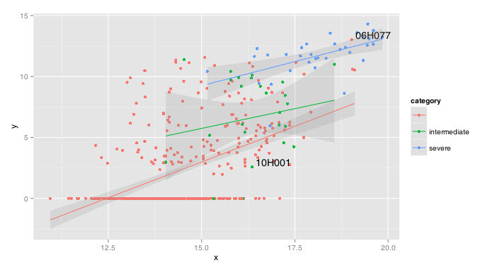
Once we have identified this point, we simply use the annotate method to add a label at these coordinates. Here is the complete function with some added functionality:
ggidentify <- function (x, y, labels, xscale=NULL, yscale=NULL) {
  depth <- downViewport('panel.3-4-3-4')
  pushViewport(dataViewport(x,y, xscale, yscale))
  pick <- grid.locator('in')
  while(!is.null(pick)) {
    pick.n <- as.numeric(pick)
    view.x <- as.numeric(convertX( unit(x,'native'), 'in' ))
    view.y <- as.numeric(convertY( unit(y,'native'), 'in' ))
    d <- min( (view.x-pick.n[1])^2 + (view.y-pick.n[2])^2 )
    w <- which.min((view.x-pick.n[1])^2 + (view.y-pick.n[2])^2)
    if (d>0.1) {
      print("Closest point is too far")
    } else {
      popViewport(n=1)
      upViewport(depth)
      print(last_plot() + annotate("text", label=labels[w], x = x[w], y = y[w],
                                   size = 5, hjust=-0.5, vjust=-0.5))
      depth <- downViewport('panel.3-4-3-4')
      pushViewport(dataViewport(x,y, xscale, yscale))
    }
    pick <- grid.locator('in')
  }
  popViewport(n=1)
  upViewport(depth)
}
Obviously, this function is still not as good as the identify we tried to emulate. For instance, there is no memory of which points are already labeled and so we might end up with a big blur when clicking multiple times. Also, picking must happen before applying other ggplot2 functions since they might cause rescaling to happen. And finally, reconverting all our data in inch at each click is definitely not optimal!
Still, we now have labels. Labels!
Leave A Comment