

When working with cancer datasets, one of the goal is sometimes to find features (mutation, clinical information, gene expression, …) associated to prognosis, i.e. features related to the probable outcome of the disease.
If that’s one of your goal, you’ll have to do a survival analysis. Survival analysis involves a set of methods to model the time at which an event of interest occurs, that event often being death. But really, any event for which the time of occurence is of interest (time of infection after a surgery, time of a graft rejection, time of rearrest of a parolee or even time a Prime Minister stays in the office –not much to do with survival, I know! –).
In a survival analysis, you try to estimate the survival function S(t), i.e. the probability that the event did not yet occur at time t. In theory, the S(t) function would look like this:
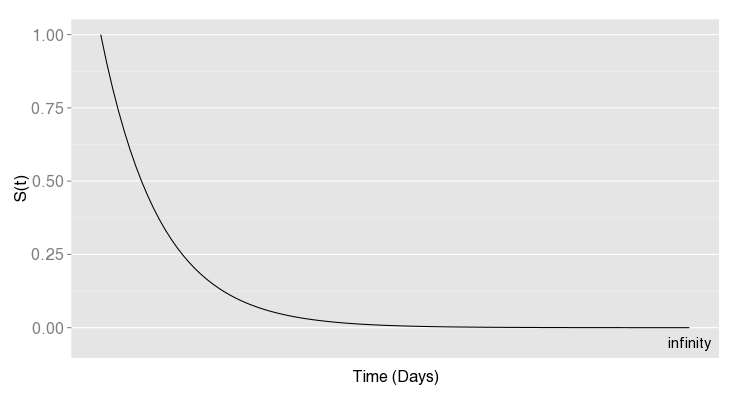
At the beginning, no one has seen the event and at time infinity (in a very long time…! ), the event happened to everyone (especially for if the event is death). This is the theoretical survival curve. I’m sure you’ve seen this kind of graph before but it was not looking like this!
In practice, one of the major problem is that you generally don’t know all the survival times. You know for a lot of your data that the event occurred at time t but for others, you don’t. You just know that the event had not occurred yet last time you collected data. It might be because the person drop out of the study, was lost in the follow up or maybe the study ended before the happening of the event. This is call censoring.
Kaplan-Meier product-limit estimator is used in practice to deal with censored data and to produce Kaplan-Meier plots. This is the kind of graph you’ve probably seen before, with each vertical mark referring to censor data.
Let’s have a closer look!
Typically, you’ll start the analysis with data in this format :
| sampleID | Overall survival (days) | Censored (deceased=1; living=0) |
| TCGA-05-4395-01 | 0 | 1 |
| TCGA-56-7822-01 | 1 | 0 |
| TCGA-85-7699-01 | 1 | 0 |
| TCGA-56-A4BW-01 | 2 | 0 |
| TCGA-85-8664-01 | 3 | 0 |
| TCGA-56-5897-01 | 3 | 0 |
| TCGA-71-8520-01 | 3 | 0 |
| TCGA-56-A5DR-01 | 4 | 0 |
| TCGA-56-A4ZK-01 | 4 | 0 |
| TCGA-77-7338-01 | 5 | 1 |
| TCGA-94-7557-01 | 5 | 1 |
The next step is to go from this format to a life-table (the conversion can be done in Excel using a matrix formula).
| Days | Deceased | Censored |
| – | – | – |
| 0 | 1 | 0 |
| 1 | 0 | 2 |
| 2 | 0 | 1 |
| 3 | 0 | 3 |
| 4 | 0 | 2 |
| 5 | 2 | 0 |
Then, you need to convert this table to the probabilities :
| Days | Deceased | Censored | Nb of subject | Cumulative survival |
| – | – | – | – | 1 |
| 0 | 1 | 0 | 11 | 10/11 * 1 = 0.909 |
| 1 | 0 | 2 | 10 | 10/10 * 0.909 = 0.909 |
| 2 | 0 | 1 | 8 | 8/8 * 0.909 = 0.909 |
| 3 | 0 | 3 | 7 | 7/7 * 0.909 = 0.909 |
| 4 | 0 | 2 | 4 | 4/4 * 0.909 = 0.909 |
| 5 | 2 | 0 | 2 | 0/2 * 0.909 = 0 |
For each time point, we compute the survival probability by dividing the number of non-event by the total. Then, we multiply the previous survival probability (t-1) to the current one. For example, for t=0, we have in total 11 subjects among which one is deceased (the event occurred). So there are 10 (11-1) subjects who did not seen the event. Hence, we divide 10/11 and multiply by the previous probability. We assume that the probability before t=0 is equal to 1.
Survival analysis are really easy to do in R and in Python (for Python’s fans, I’ve already introduced the package lifelines here). You’ll find a list of survival related packages here. In R, it’s as simple as this :
library(survival)
data(lung)
Y = Surv(lung$time, lung$status)
s = survfit(Y~1)
plot(s)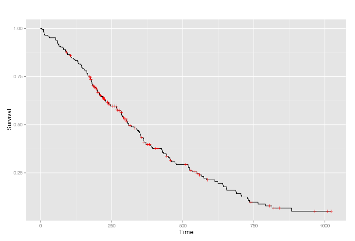
There are also a couple of options (SurvCurv or Oasis) to do the survival analysis online. They work well but require that you submit the data in the life-table format.
Leave A Comment