

Mariana was previously introduced in this blog by Geneviève in her May post Machine learning in life science.
The Mariana codebase is currently standing on github at the third release candidate before the launch of the stable 1.0 release. This new version incorporates a large refactorization effort as well as many new features (a complete list of the changes found in the 1.0 version can be found in the changelog). I am taking this opportunity to present here a small tutorial on extending the functionalities of Mariana 1.0.
Implementing a “Siamese” Neural Network
The Mariana documentation is ripe with use cases for the various networks already implemented within Mariana, but what about functionalities that aren’t yet implemented? Extending Mariana can be done with minimal effort. Let’s take the “Siamese” network described in Signature Verification using a “Siamese” Time Delay Neural Network as example [1].
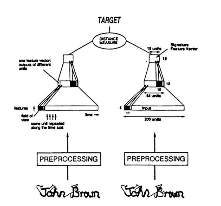
In this example, the network attempts to identify forged signatures. When faced with a pair of signatures, the network attempts to identify if both signatures are genuine or if one of the signatures is a forgery. To do so, the network is composed of two parallel feed-forward networks with tied weights. The cosine similarity measure of the output of both network is used as the distance measure between both inputs. A threshold is selected to determine whether the pair is composed of both genuine or genuine and forged signatures.
$ \text{Cosine Similarity} = \cos(\theta) = {\mathbf{A} \cdot \mathbf{B} \over \|\mathbf{A}\| \|\mathbf{B}\|} = \frac{ \sum\limits_{i=1}^{n}{A_i B_i} }{ \sqrt{\sum\limits_{i=1}^{n}{A_i^2}} \sqrt{\sum\limits_{i=1}^{n}{B_i^2}} }$
In order to implement such a network in Mariana, we must add a new output layer. In order to do so, two modifications must be done to the base Mariana output class : 1) manage connections between the layers of the two branches of the network and 3) define the cosine similarity measure at the output.
Let’s get started with our new layer. This layer, aptly named Siamese, will need to abstract the base class for all output layers in Mariana, Output_ABC.
import theano.tensor as tt
from Mariana.layers import Output_ABC
class Siamese(Output_ABC):
    def __init__(self, **kwargs):
        Output_ABC.__init__(self, size=1, **kwargs)
        self.targets = tt.ivector(name="targets_" + self.name)
        self.inpLayers = []
Our Siamese layer must also implement some restrictions on its connections. Here, the function _femaleConnect will enforce a maximum of 2 input connections and will ensure that the outputs of these two input layers are of the same size.
    def _femaleConnect(self, layer):
        if self.nbInputs is None:
            self.nbInputs = layer.nbOutputs
        elif self.nbInputs != layer.nbOutputs:
            raise ValueError("All inputs to layer %s must have the same size, \
got: %s previous: %s" % (self.name, layer.nbOutputs, self.nbInputs))

        if len(self.inpLayers) > 2:
            raise ValueError("%s cannot have more than 2 input layers." % (self.name))
        self.inpLayers.append(layer)
Manipulation of the outputs of our layer is described in the function _setOutputs. This is where the cosine similarity will be implemented.
    def _setOutputs(self):
        """Defines self.outputs and self.testOutputs"""

        if len(self.inpLayers) != 2:
            raise ValueError("%s must have exactly 2 input layers." % (self.name))

        num = tt.sum(self.inpLayers[0].outputs * self.inpLayers[1].outputs, axis=1)
        d0 = tt.sqrt(tt.sum(self.inpLayers[0].outputs**2, axis=1))
        d1 = tt.sqrt(tt.sum(self.inpLayers[1].outputs**2, axis=1))

        num_test = tt.sum(self.inpLayers[0].testOutputs * self.inpLayers[1].testOutputs, axis=1)
        d0_test = tt.sqrt(tt.sum(self.inpLayers[0].testOutputs**2, axis=1))
        d1_test = tt.sqrt(tt.sum(self.inpLayers[1].testOutputs**2, axis=1))

        self.outputs = num / (d0 * d1)
        self.testOutputs = num_test / (d0_test * d1_test)
Nearly done! Now that we have our Siamese output layer, let’s move on to constructing our network.
As it was for previous Mariana versions, describing the structure and connections of the network remains childsplay. Once instantiated, the network components can be strung together using the > operator. This detail allows for rapid network prototyping and the easy creation of many differents network structures such as forks, fusions and loops (a complete implementation of recurrent neural networks are, however, not yet implemented in Mariana).
Our network will be trained by gradient descent with a learning rate of 0.01. A mean squared error is used as the cost function.
ls = MS.GradientDescent(lr=0.01)
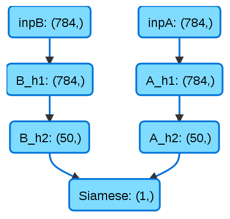
cost = MC.MeanSquaredError()The layers of the network must now be instantiated. Two branches, A and B, with one input layer (_i) and two hidden layers (_h1, _h2), are introduced which use a rectifier (MA.ReLU) as activation function as well as a bit of L2 regularization (MR.L2). The size of each layer is passed as the first argument. Finally, our Siamese output layer is instantiated and linked up with the other layers using the > operator.
import Mariana.activations as MA
import Mariana.layers as ML
import Mariana.costs as MC
import Mariana.regularizations as MR
import Mariana.scenari as MS

A_i = ML.Input(28 * 28, name='inpA')
A_h1 = ML.Hidden(28 * 28, activation=MA.ReLU(), regularizations=[MR.L2(0.01)], name='A_h1')
A_h2 = ML.Hidden(50, activation=MA.ReLU(), regularizations=[MR.L2(0.01)], name='A_h2')

B_i = ML.Input(28 * 28, name='inpB')
B_h1 = ML.Hidden(28 * 28, activation=MA.ReLU(), regularizations=[MR.L2(0.01)], name='B_h1')
B_h2 = ML.Hidden(50, activation=MA.ReLU(), regularizations=[MR.L2(0.01)], name='B_h2')

o = Siamese(learningScenario=ls, name='Siamese', costObject=cost)

network = A_i > A_h1 > A_h2 > o
network = B_i > B_h1 > B_h2 > o
All that remains to do is to tie the weights of the hidden layers of both branches. We must first instantiate the network in order for the weights to be initialized with the same values.
network.init()
A_h1.W = B_h1.W
A_h2.W = B_h2.W
The saveHTML function offers us a peak at the final structure of our network:
Version 1.0 is expected to be released in the coming months. Keep an eye out on the github page for the newest updates!
I’d like to thank Tariq Daouda, author of Mariana, for his help in writing this post.
References
[1] Bromley, Jane, et al. “Signature verification using a “Siamese” time delay neural network.” International Journal of Pattern Recognition and Artificial Intelligence 7.04 (1993): 669-688.
Leave A Comment