

In 2016, Bray et al. introduced a new k-mer based method to estimate isoform abundance from RNA-Seq data. Their method, called kallisto, provided a significant improvement in speed and memory usage compared to the previously used methods while yielding similar accuracy. In fact, kallisto is able to quantify expression in a matter of minutes instead of hours. Since it is so light and convenient, kallisto is now often used to quantify expression in the form of TPM. But how does it work?
Standard (previous) methods for quantifying expression relied on mapping, i.e. on the alignment of RNA-Seq sequenced reads to a reference genome. Reads are assigned to a position in the genome and the gene or isoform expression values are derived by counting the number of overlapping reads (overlapping the features of interest).
The idea behind kallisto is to rely on a pseudoalignment which does not identify the positions of the reads in the transcripts, only their potential transcripts of origin. Thus, it avoids doing an alignment of each read to a reference genome. It actually only uses the transcriptome sequences (not the whole genome).
Before analyzing any sample, it is essential to construct a kallisto index. kallisto first builds a colored de Bruijn graph (T-DBG) from all the k-mers found in the transcriptome. Each node of the graph corresponds to a k-mer (a small sequence of k bases) and retains the information about transcripts in which they can be found in the form of a color. The linear stretches in the graph having the same coloring correspond to contigs or transcripts. Once the T-DBG is built, kallisto stores a mapping between each k-mer and its transcript(s) of origin along with the position within the transcript(s). This step is done only once and is dependent on a provided annotation file (containing the sequences of all the transcripts in the transcriptome).
Then for a given sequenced sample, kallisto decomposes each read into its k-mers and uses those k-mers to find a path covering in the T-DBG. This path covering of the transcriptome graph, where a path corresponds to a transcript, generates k-compatibility classes for each k-mer, i.e. sets of potential transcripts of origin on the nodes. The potential transcripts of origin for a read (not a k-mer here) can be obtained using the intersection of its k-mers k-compatibility classes. To make the pseudoalignment faster, kallisto skips redundant k-mers because neighboring k-mers often belong to the same transcripts. Figure1, from the paper, summarizes these different steps.
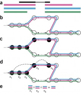
Figure1. Overview of kallisto. The input consists of a reference transcriptome and reads from an RNA-seq experiment. (a) An example of a read (in black) and three overlapping transcripts with exonic regions as shown. (b) An index is constructed by creating the transcriptome de Bruijn Graph (T-DBG) where nodes (v1, v2, v3, … ) are k-mers, each transcript corresponds to a colored path as shown and the path cover of the transcriptome induces a k-compatibility class for each k-mer. (c) Conceptually, the k-mers of a read are hashed (black nodes) to find the k-compatibility class of a read. (d) Skipping (black dashed lines) uses the information stored in the T-DBG to skip k-mers that are redundant because they have the same k-compatibility class. (e) The k-compatibility class of the read is determined by taking the intersection of the k-compatibility classes of its constituent k-mers. [From Bray et al. Near-optimal probabilistic RNA-seq quantification, Nature Biotechnology, 2016.]
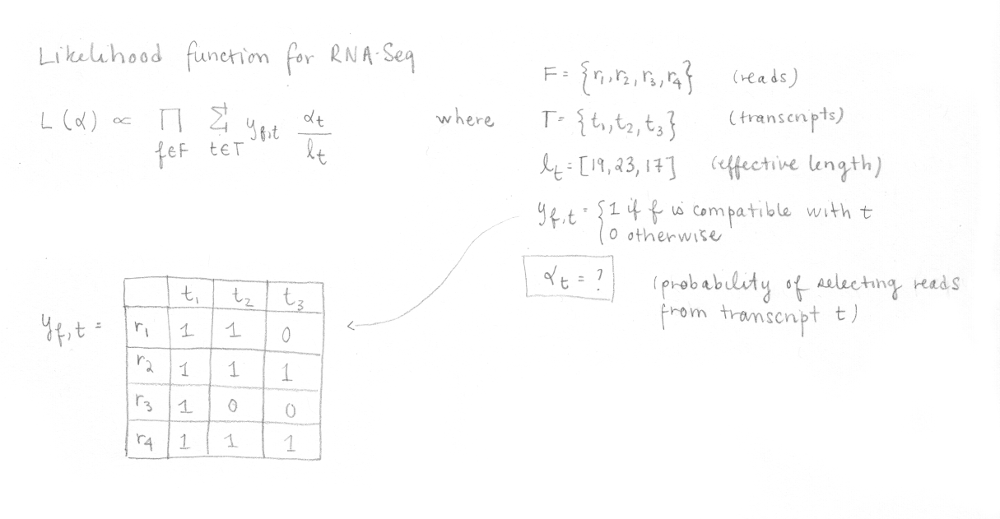
Then, kallisto optimize the following RNA-Seq likelihood function using the expectation-maximization (EM) algorithm.
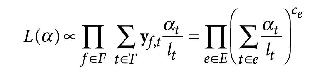
In this function, F is the set of fragments (or reads), T is the set of transcripts, lt is the (effective) length of transcript t and yf,t is a compatibility matrix defined as 1 if fragment f is compatible with t and 0 otherwise. The parameters αt are the probabilities of selecting reads from transcript t. These αt are the parameters of interest since they represent the isoforms abundances or relative expressions.
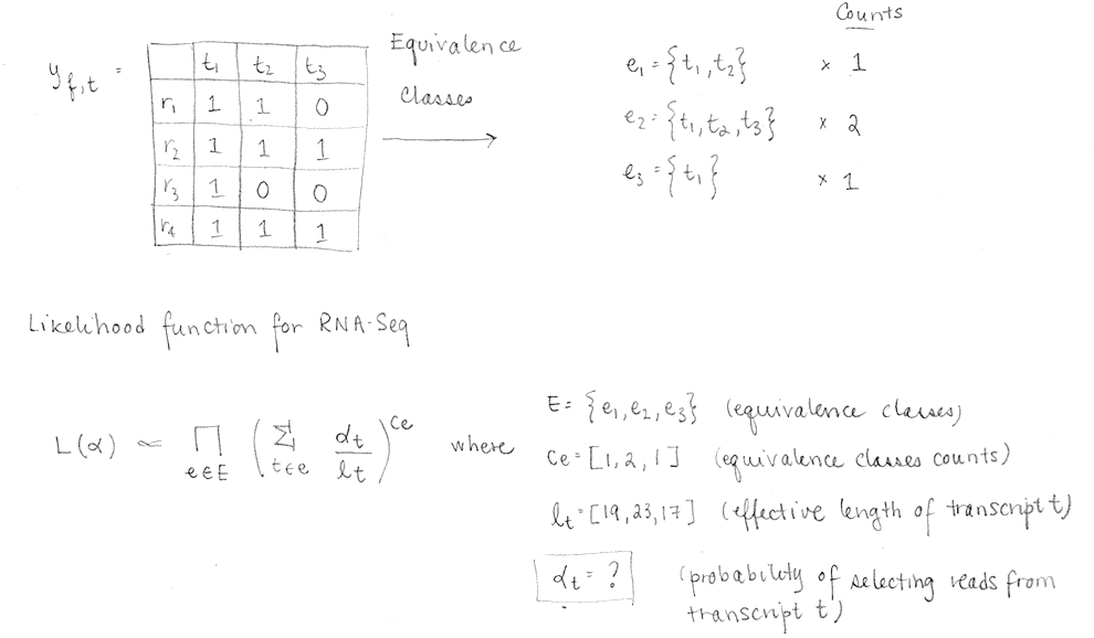
To make things faster, the compatibility matrix is collapsed (factorized) into equivalence classes. An equivalent class consists of all the reads compatible with the same subsets of transcripts. The EM algorithm is applied to equivalence classes (not to to reads). Each αt will be optimized to maximize the likelihood.
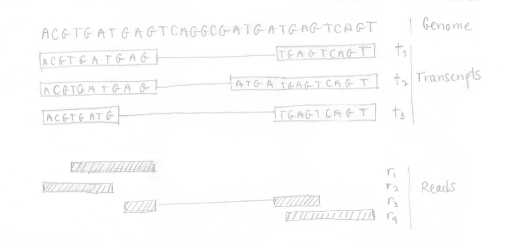
Practically, we can illustrate the different steps involved in kallisto using a small example. Starting from a tiny genome with 3 transcripts, assume that the RNA-Seq experiment produced 4 reads as depicted in the following image.
If you remember, the first step is to build the T-DBG graph and the kallisto index. All transcript sequences are decomposed into k-mers (here k=5) to construct the colored de Bruijn graph. I did not represent all the nodes/k-mers in the drawing but you can imagine there are more nodes aligned (not at a branching site). The idea is that each different transcript will lead to a different path in the graph. The strand is not taken into account, kallisto is strand-agnostic.
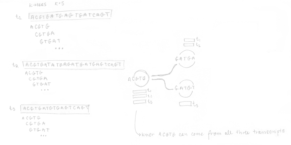
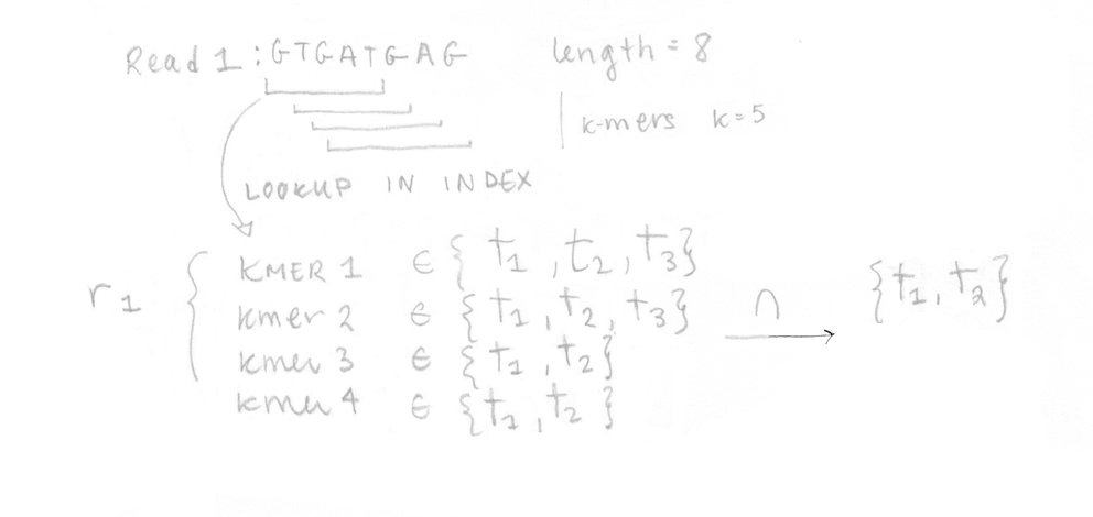
Once the index is built, the 4 reads of the sequenced sample can be analysed. They are decomposed into k-mers (k=5 here too) and the pre-built index is used to determine the k-compatibility classes of each k-mer. Then, the k-compatibility class of each read is computed. For example, for read 1, the intersection of all the k-compatibility classes of its k-mers suggests that it might come from transcript 1 or transcript 2.
This is done for the four reads enabling us to build the compatibility matrix yf,t which is part of the likelihood function for RNA-Seq that we want to maximize. I’ve written the equation with its different parts explained. In our case, applying the EM algorithm to four reads is not a problem, but in reality, it would be too slow to apply it on millions of reads.
Thus, the compatibility matrix yf,t is collapsed into equivalence classes and a count is computed for each class (how many reads are represented by this equivalence class). The EM algorithm uses this collapsed information to maximize the equivalent RNA-Seq likelihood function and optimize the αt , which are the values that we want to determine.
The EM algorithm will change αt as to maximize L(α), i.e. it will try different values of probabilities for each transcript in order to get the highest likelihood possible. And it does it in a wise way allowing it to converge. I did not run the EM algorithm, but to give you an intuition, let’s look at this small example. In this example, initializing the three probabilities αt (i.e. probabilities of selecting reads from each transcript) to an equal value of 0.33 gives a L(α) of 8.4e-05.
If I change the abundance values to [0.98, 0.01, 0.01] (more chances of coming from transcript 1) instead of [0.33, 0.33, 0.33], I now get L(α) of 4.2e-4, which is greater than 8.4e-05. [0.05, 0.05, 0.9] gives 2.2e-06. You get the idea….
[0.33, 0.33, 0.33] ==> 8.4e-05
[0.45, 0.15, 0.4] ==> 0.00011
[0.98, 0.01, 0.01] ==> 0.00042
[0.9, 0.05, 0.05] ==> 0.00037
[0.05, 0.9, 0.05] ==> 1.5e-05
[0.05, 0.05, 0.9] ==> 2.2e-06
[0.15, 0.45, 0.4] == >3.3e-05
In this example, considering the four reads, it is likely that the reads come from transcript 1 which would be the most abundant of all three transcripts. We would consider [0.98, 0.01, 0.01] to be the relative abundance of the transcripts. In kallisto, the EM algorithm stops when for every transcript t, αtN > 0.01, where N is the total number of reads, changes less than 1%.
While being a nice paper, the kallisto paper is not super easy to understand. I hope I was able to help a little bit in the understanding of how this popular tool works.
Merci pour cette explication!
Hello,
Thanks for the wonderful explanation. Could you please elucidate the EM step?
Thank you.
Very clear explanation. Excellent example. Thanks a lot for this post. It really helped me a lot
But I have a doubt. How they are taking the probability values? Just randomly or based on any reference. If the probabilities are assumed according to the equivalance matrix, if should follow that 2:1:1 ratio. If that is the case [0.33 0.33 0.33] is not a right way to assume probabilities. That is why I am getting this doubt whether the probability assumption is random or it is based on equivalance matrix ratios?
Hi Krishna, thank you for the feedback. Actually, the values [0.33,0.33,0.33] mentioned in the post were an arbitrary choice on my part to give an intuition of how the EM algorithm works. Going into the details of the EM algorithm would have been a lot for one post, but I nevertheless tried to explain at a very high level how it works. That may be the source of the confusion.
Thanks a lot. Can you please explain EM steps too?
I am really thankful to you for clearly explaining how Kallisto algorithm works. It removedb many doubts I had when I read the original paper. You have brilliantly explained it with specific example. Thanks a lot.
Thank you!
what is output of kallisto and in which format is it?