Applying statistical methods is a large part of the work of a bioinformatician. Apart from some more classical techniques, machine learning algorithms are also regularly applied to clinical and biological data (notably, clustering techniques such as k-means).
Some techniques such as artificial neural networks have recently found great success in areas such as image recognition and natural language processing. However, these techniques do not perform as well on small datasets with high dimensionality, a problem known as “the curse of dimensionality“. These types of datasets are, unfortunately, a common occurrence at the platform.
This drawback can be mitigated by adding synthetic data. To do so, data is artificially created from the original data by introducing a small amount of noise while trying to preserve the defining characteristics of each sample. The inflation of the size of the dataset by the addition of synthetic data can, in some cases, help with performance and generalization.
Generating Synthetic RNASeq Samples
An RNASeq dataset from a gene expressions analysis project was chosen as candidate for a synthetic data upgrade.
In this case, the new samples were generated by a simple bootstrap on the reads of the aligned (tophat) BAM file. In other words, for a sample with N reads, N reads are picked randomly from the original sample with replacement. The output therefore contains different read counts as some will be picked more often than others and some will be left out altogether.
This feat is accomplished by a small Python script invoking samtools through the Pysam interface. After completion, the output file must then be repassed through the gene expression quantification pipeline (cuffquant / cuffnorm).
Here is a stripped down version of the script in question.
import pysam
import random

bam_in = "original.bam"
bam_out = "synthetic.bam"

bam = pysam.AlignmentFile(bam_in)
read_table = {}

for idx, read in enumerate(bam.fetch()):
    read_table[read.qname] = 0

# Bootstrap
nb_reads = len(read_table)
read_list = read_table.keys()
for _ in range(0, nb_reads):
    pick = read_list[random.randrange(nb_reads)]
    read_table[pick] += 1

# Build the new file based on the bootstrapping
new_bam = pysam.AlignmentFile(bam_out, "wbu", template=bam)
for idx, read in enumerate(bam.fetch()):
    for x in range(0, read_table[read.qname]):
        read.qname += "_%s" % x
        new_bam.write(read)

new_bam.close()
Results
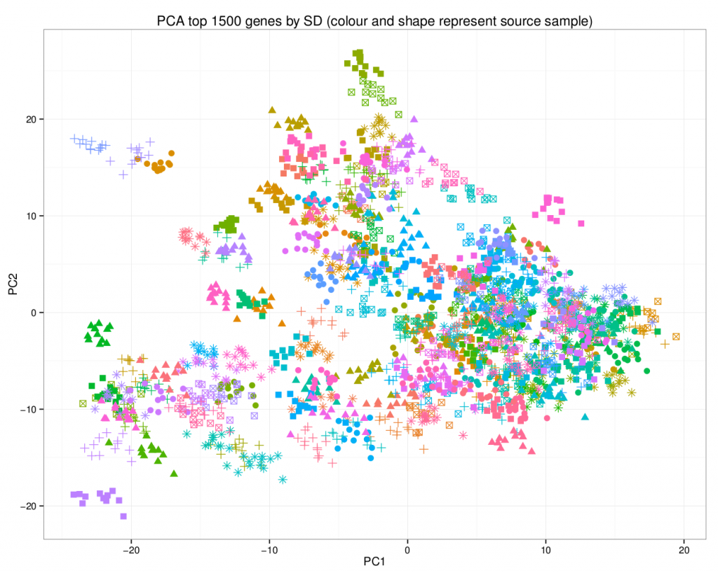
A principal component analysis of the final dataset allows us to visualize the addition of the synthetic data.
In this plot, the synthetic data points are of the same colour / shape combination as their original counterpart. Note how they share the same area on the graph.


Leave A Comment