

Working with all sorts of data, it happens sometimes that we want to predict the value of a variable which is not numerical. For those cases, a logistic regression is appropriate. It is similar to a linear regression except that it deals with the fact that the dependent variable is categorical.
Here is the formula for the linear regression, where we want to estimate the parameters beta (coefficients) that fit best our data :
\begin{equation}
Y_i = \beta_0 + \beta_1 X_i + \epsilon_i
\end{equation}
Well, in a logistic regression, we are still estimating the parameters beta but for :
\begin{equation}
y = \left\{\begin{matrix}1\: \: \: \: Y_i = \beta_0 + \beta_1 X_i + \epsilon_i > 0
\\
0\: \: \: \:else
\end{matrix}\right.
\end{equation}
Here, y is not linearly dependent on x. Let’s look at an example.
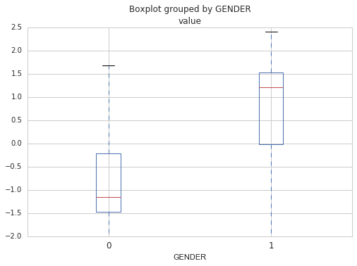
Predicting the sex from the gene expression profiles
When building a model from expression data, I usually try to build a model that can predict the sex. This serves as a great control, since it is a very easy task. Looking at just a few genes from the chromosome Y is enough to assess the sex.
For my example, I have decided to use The Genotype-Tissue Expression (GTEx) RPKM dataset. GTEx Portal allows you to look at transcriptomic data and genetic association across several tissues of healthy deceased donors. The V6p release contains the 8555 samples surveying 53 tissues from 544 post-mortem donors. You should have a look at their portal, it’s really interesting and user-friendly.
Since GTEx’s dataset is quite big (56238 rows by 8555 columns), I have used python to do the logistic regression using functions from the scikit-learn package. If you have a smaller dataset, the R function glm(formula, data=mydata, family='binomial') is what you are looking for.
So, here we go. The first steps are : 1) loading the RPKM matrix, the sample annotations and the subject annotations, 2) log-transforming the RPKM values (log10(RPKM+0.01)) 3) filtering the genes to keep the 10,000 most variable ones. I’m keeping a little less than 20% of the genes for the example but it is an arbitrary decision.
| SMCENTER | SMTS | SMTSD | SUBJECT | |
|---|---|---|---|---|
| GTEX-1117F-0003-SM-58Q7G | B1 | Blood | Whole Blood | GTEX-1117F |
| GTEX-1117F-0003-SM-5DWSB | B1 | Blood | Whole Blood | GTEX-1117F |
| GTEX-1117F-0226-SM-5GZZ7 | B1 | Adipose Tissue | Adipose – Subcutaneous | GTEX-1117F |
| GTEX-1117F-0426-SM-5EGHI | B1 | Muscle | Muscle – Skeletal | GTEX-1117F |
| GTEX-1117F-0526-SM-5EGHJ | B1 | Blood Vessel | Artery – Tibial | GTEX-1117F |
Table1. Example of the data
When trying to predict something, it is recommended to always work with a training and a test sets. You build your model using the training set and than you assess it’s performance on the test set. All scikit-learn functions are designed to work in this fashion.
from sklearn.linear_model import LogisticRegression
from sklearn import metrics, cross_validation
from sklearn.cross_validation import train_test_split
from sklearn.cross_validation import cross_val_score

# X is the sample by gene matrix,
# Y is a vector containing the gender of each sample
# 0.3 means I want 30% of the data in the test set and 70% in the training set

X_train, X_test, y_train, y_test = train_test_split(X, Y, test_size=0.3, random_state=0)

# Those parameters try to restrain the variables used in the model
model = LogisticRegression(penalty='l2', C=0.2)
model.fit(X_train, y_train)

# Apply the model on the test set
predicted = model.predict(X_test)
probs = model.predict_proba(X_test)
That’s it! Once the model has converged, I can look at the predictions on the training and test set, to see how well it did. Since there was 62.3% of males in the test set (that close to the proportion of males in the whole dataset), the model needs to be right more than 62.3% of the time to say that it is performing well. Otherwise, it could just say ‘male’ all the time (without using the actual gene expression data) and it would be right 62.3% of the time. For this example, the model had an accuracy of 100%. It made the right call for all the samples.
Then, by looking at the beta coefficients, I can identify which genes are important for predicting the sex. Those would be the genes having the greater or smallest coefficients. Top four genes includes : RPS4Y1 (coefficient of 1.34), KDM5D (1.27), DDX3Y (1.25) and XIST (-1.25). Note that XIST is the only one that looks specific to female.
Note that you should always do cross-validation to be sure that the model is not specific to your dataset (that is does not overfit). The goal of building a predictive model is after all to be able to reuse it on new data, so it needs to be able to generalize. Cross-validation implies building the model several times using different training and test sets and averaging the scores to get a sense of its real performance. In the code below, the model is built 10 times each time using a different training set and test set. The mean score for the 10 iterations tells us if the model is good at generalization.
# evaluate the model using 10-fold cross-validation
scores = cross_val_score(LogisticRegression(penalty='l2', C=0.2), xx.T, Y, scoring='accuracy', cv=10)
Predicting the tissue from the gene expression profiles
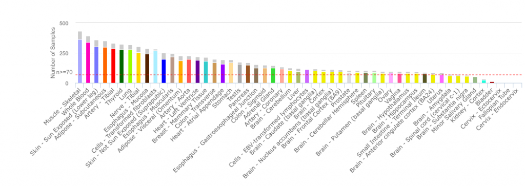
Now, for fun, I can try to derive a model that will predict the tissue. I say for fun because I’ll only look at one model (not cross-validated) and because of the different number of samples in each category of tissue. One category has 1259 samples and the other only 6. This might need to be address.
So, there are 31 high level tissue types in the dataset, the two most represented being Brain and Skin, respectively 14.7% and 10.4% of the samples. Using the same code and matrix as before, only changing the vector Y – which is my dependent variable that I want to predict-, I get a good model which is right 99.3 % of the time. It made 18 errors on a total of 2567 predictions. Interestingly, a number of the errors involved female tissues, which may be related to the fact that female samples are under-represented in the dataset!
| Predicted | Real |
|---|---|
| Stomach | Vagina |
| Nerve | Adipose Tissue |
| Esophagus | Stomach |
| Colon | Small Intestine |
| Esophagus | Stomach |
| Esophagus | Stomach |
| Colon | Esophagus |
| Skin | Vagina |
| Uterus | Fallopian Tube |
| Adipose Tissue | Breast |
| Ovary | Fallopian Tube |
| Skin | nan |
| Blood Vessel | Uterus |
| Adipose Tissue | Stomach |
| Stomach | Colon |
| Esophagus | Stomach |
| Heart | Blood Vessel |
| Adipose Tissue | Fallopian Tube |
Table2. Errors made by the model.
Leave A Comment