

Understanding dimensionality reduction
If you use large datasets (transcriptomes, whole genome sequencing, proteomes), sooner or later you will stumble across something called Principal Components Analysis (PCA). PCA is a dimensionality reduction, a family that encompasses many techniques that do just that: reduce the dimensionality.
But what does that mean? What are dimensions and why would we want to reduce their number?
How about we deal with these questions through an example?
The problematic
Say we have a hypothetical transcriptome, of a very primitive species, that has a total of 3 genes in its genome. Some of these individuals were treated with some drug and you are observing the changes in gene expression. If we plot all possible combinations of gene expressions we get the following set of graphs. General note: dimensions we refer to are here just a fancy word for genes.
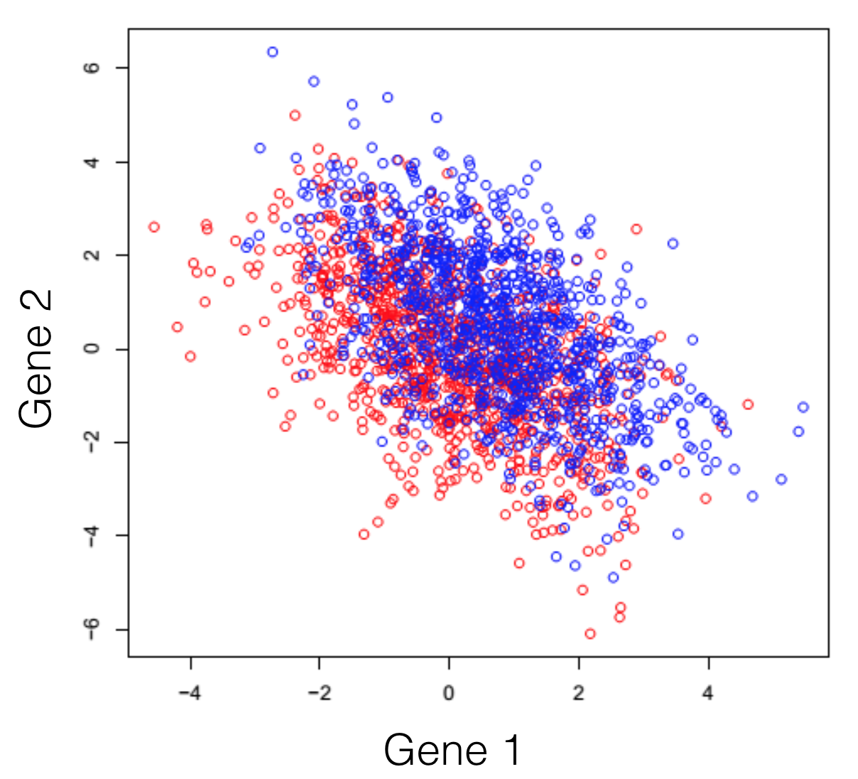
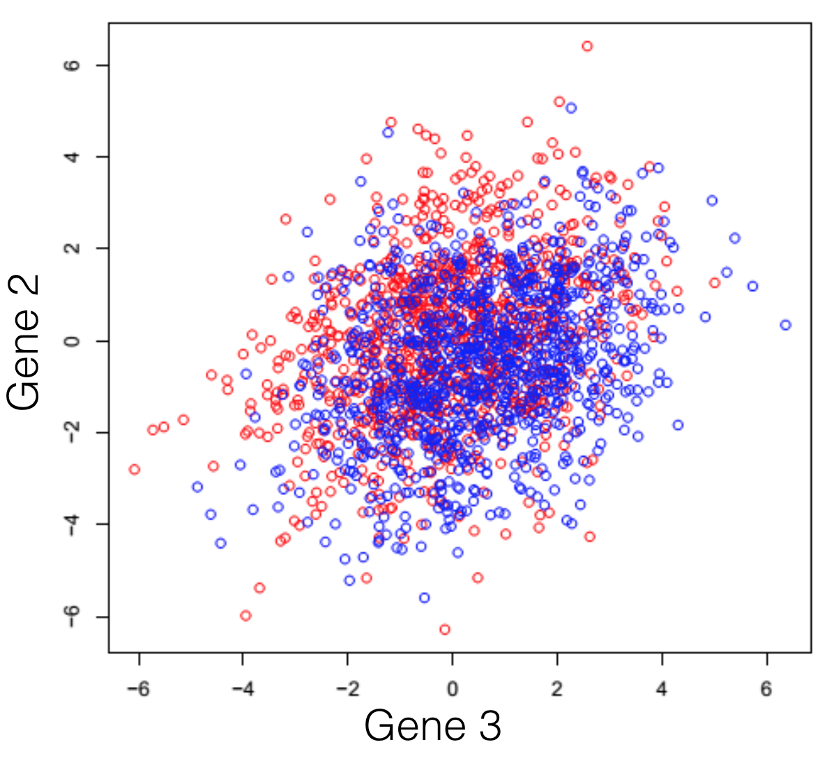
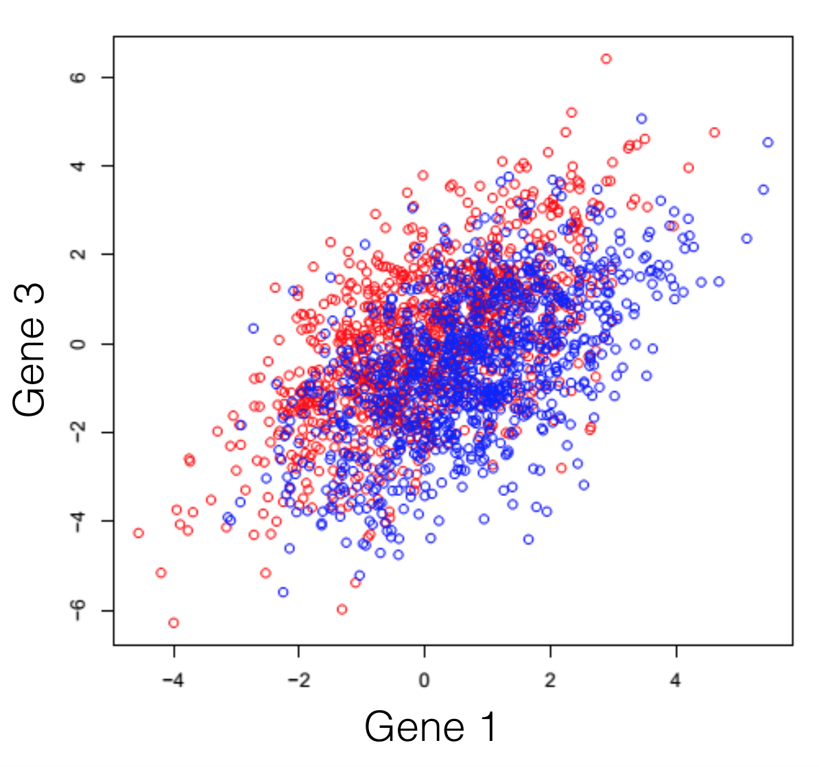
And here we see that there is a trend, but it seems to be distributed over the organism’s 3 genes and impossible to extract. This trend, although visible to the naked eye, can be distilled from the data, using a dimensionality reduction technique. Reducing dimensions doesn’t mean discarding some and keeping others. This family of methods attempts to remove redundancies, by creating a new dimension set, that explains better the observed samples in the dataset. In the following post (and others to come), I will provide an intuitive explanation of what each dimensionality reduction does.
Principal Components Analysis
Specifically for the PCA, the point is to create a new system of coordinates that does its best to explain the variance of the samples. In other words, the PCA will look for one direction in the dataset, that separates the most the samples. Then, it will look for another dimension, the second “most separating one”.
There is however a technical catch: all new dimensions need to be orthogonal to each other. Orthogonal refers to a right angle. The choice to have all new dimensions located at a right angle from each other may be attributed to the fact that in the original set of dimensions, they are at a right angle from one another.
Sometimes PCA is referred to as a rotation. The rotation is done in the dataset space, to find that first dimension that separates best the samples. You will notice in the gif below (click the button to see the animation), that after a rotation, the two groups from our fictive dataset can be easily separated.

If you had to explain how the rotation is done, intuitively you would say that the rotation is a certain angle, at which we have rotated the space. Knowing that you can explain an angle as a linear combination of two dimensions, the rotation we have created can be defined as a linear combination of the dimensions.
Another very important observation is that suddenly, you don’t need to represent your dataset in 3d (with the gene expression values). You could easily draw the dataset in 2d (where each dimension is a linear combination of the inputs), as it is represented on the screen.
thanks Assya